
The Hawaii-Pacific Islands Region includes the State of Hawai‘i, American Samoa, Guam, the Commonwealth of the Northern Mariana Islands, and various uninhabited remote Pacific Islands. The combined coastline is 2,930.5 kilometers, and the combined land area is 17,842 square kilometers. The population density in this region is relatively high, especially in the State of Hawai’i. High density coastal populations often place inordinate stressors on coastal ecosystems leading to detrimental effects on flora and fauna i.e. point source and non point source pollution.
The region is home to the critically endangered Hawaiian monk seal - only 1,400 remain - as well as other iconic and threatened species such as green sea turtles, spinner dolphins, false killer whales, and humpback whales. Coral reefs support about 25% of this region's marine life, but these also face challenges from natural event impacts and human activities, such as coral bleaching and disease, marine debris, pollution, and ocean acidification.
Over 90% of the ocean-related employment in this region is in the tourism and recreation sector.
Understanding the Time series plots
Time series plots show the changes in each indicator as a function of time, over the period 1980-present. Each plot also shows horizontal lines that indicate the median (middle) value of that indicator, as well as the 10th and 90th percentiles, each calculated for the entire period of measurement. Time series plots were only developed for datasets with at least 10 years of data. Two symbols located to the right of each plot describe how recent values of an indicator compare against the overall series. A black circle indicates whether the indicator values over the last five years are on average above the series 90th percentile (plus sign), below the 10th percentile (minus sign), or between those two values (solid circle). Beneath that an arrow reflects the trend of the indicator over the last five years; an increase or decrease greater than one standard deviation is reflected in upward or downward arrows respectively, while a change of less than one standard deviation is recorded by a left-right arrow.

Pacific Decadal Oscillation (PDO)
During the last five years, the PDO indicator has trended downward, shifting from positive phase to negative phase in 2019.
Values correspond to Index scores
Description of time series:
Positive PDO values typically mean cool surface water conditions in the interior of the North Pacific Ocean and warm surface waters along the North American Pacific Coast while negative PDO conditions typically mean warm surface water conditions in the interior to the North Pacific Ocean and cool surface waters along the North American Pacific Coast. During the last five years, the PDO indicator has trended downward, shifting from positive phase to negative phase in 2019.
Description of Pacific Decadal Oscillation (PDO):
The Pacific Decadal Oscillation (PDO) is a long-term pattern of Pacific climate variability that comprises multiple physical forcing mechanisms. The extreme phases of this climatic condition are classified as warm or cool, based on deviations from average ocean temperature in the northeast and central North Pacific Ocean. When the PDO has a positive value, sea surface temperatures are below average (cool) in the interior North Pacific and warm along the Pacific Coast. When the PDO has a negative value, the climate patterns are reversed, with above average sea surface temperatures in the interior and sea surface temperatures below average along the North American coast. On shorter timescales a positive (negative) PDO is often related to El Niño (La Niña). The PDO waxes and wanes on longer timescales as well; warm and cold phases may persist for decades. Major changes in northeast Pacific marine ecosystems have been correlated with phase changes in the PDO. Warm phases have seen enhanced coastal ocean biological productivity in Alaska and inhibited productivity off the west coast of the United States, while cold PDO phases have seen the opposite, north-south pattern of marine ecosystem productivity. We present data from the Pacific Islands, Alaska, and California Current regions
Data Background:
Climate indicator data was accessed from the NOAA NCEI (https://www.NCEI.noaa.gov/teleconnections/pdo/data.csv). The data plotted are unitless and based on Sea Surface Temperature anomalies averaged across a given region.
East Pacific - North Pacific Teleconnection Pattern Index
During the last five years, the EP-NP indicator has shifted from mostly positive to mostly negative.
Values correspond to Index scores
Description of time series:
Positive EP-NP values mean above-average surface temperatures over the eastern North Pacific, and below-average temperatures over the central North Pacific and eastern North America and the opposite for negative EP-NP values. During the last five years, the EP-NP indicator has shifted from mostly positive to mostly negative.
Description of East Pacific/ North Pacific Teleconnection Pattern Index:
The East Pacific/ North Pacific Teleconnection Pattern Index is a measure of climate variability. Positive EP-NP values mean above-average surface temperatures over the eastern North Pacific, and below-average temperatures over the central North Pacific and eastern North America and the opposite for negative EP-NP values.
This climate condition impacts people and ecosystems across the globe and each of the indicators presented here. Interactions between the ocean and atmosphere alter weather around the world and can result in severe storms or mild weather, drought, or flooding. Beyond “just” influencing the weather and ocean conditions, these changes can produce secondary results that influence food supplies and prices, forest fires and flooding, and create additional economic and political consequences. The positive phase of the EP-NP pattern is associated with above-average surface temperatures over the eastern North Pacific, and below-average temperatures over the central North Pacific and eastern North America. The main precipitation anomalies associated with this pattern reflect above-average precipitation in the area north of Hawaii and below-average precipitation over southwestern Canada
Data Background:
Climate indicator data was accessed from NOAA NCEP (https://ftp.cpc.ncep.noaa.gov/wd52dg/data/indices/epnp_index.tim). The data plotted are unitless anomalies.
El Niño-Southern Oscillation (Oceanic Niño Index)
After an El Nino event that spanned much of 2023, conditions transitioned to ENSO neutral in the spring of 2024 and have remained neutral since then.
Values correspond to Index scores
Description of time series:
The Oceanic Niño Index (ONI) is NOAA’s primary index for monitoring the El Niño-Southern Oscillation climate pattern. It is based on Sea Surface Temperature values in a particular part of the central equatorial Pacific, which scientists refer to as the Niño 3.4 region. Positive values of this indicator, greater than +0.5, indicate warm El Niño conditions, while negative values, less than -0.5, indicate cold La Niña conditions. Values between +0.5 and -0.5 are considered ENSO neutral. The ONI shifted from La Nina conditions to neutral conditions in early 2023, and with continued sea-surface warming now indicate that an El Nino has begun.
Description of El Niño-Southern Oscillation (ENSO):
El Niño and La Niña are opposite phases of the El Niño-Southern Oscillation (ENSO), a cyclical condition occurring across the Equatorial Pacific Ocean with worldwide effects on weather and climate. During an El Niño, surface waters in the central and eastern equatorial Pacific become warmer than average and the trade winds - blowing from east to west - greatly weaken. During a La Niña, surface waters in the central and eastern equatorial Pacific become much cooler, and the trade winds become much stronger. El Niños and La Niñas generally last about 6 months but can extend up to 2 years. The time between events is irregular, but generally varies between 2-7 years. To monitor ENSO conditions, NOAA operates a network of buoys, which measure temperature, currents, and winds in the equatorial Pacific.
This climate pattern impacts people and ecosystems around the world by affecting large scale areas of tropical convection, and by extension, the jet streams. Interactions between the ocean and atmosphere alter weather globally and can result in severe storms or mild weather, drought or flooding. Beyond “just” influencing the weather and ocean conditions, these changes can produce secondary results that influence food supplies and prices, forest fires and flooding, and create additional economic and political consequences. For example, along the west coast of the U.S., warm El Niño events are known to inhibit the delivery of nutrients from subsurface waters, suppressing local fisheries. El Niño events are typically associated with fewer hurricanes in the Atlantic while La Niña events typically result in greater numbers of Atlantic hurricanes.
Data Background:
ENSO ONI data was accessed from NOAA’s Climate Prediction Center (https://origin.cpc.ncep.noaa.gov/products/analysis_monitoring/ensostuff/ONI_v5.php). The data are plotted in degrees Celsius and represent Sea Surface Temperature anomalies averaged across the so-called Niño 3.4 region in the east-central tropical Pacific between 120°-170°W and 5°S-5°N .
Multivariate El Niño-Southern Oscillation Index (MEI)
The MEI indicator shifted from neutral to negative in the spring of 2024 and has been indicating La Nina conditions since then.
Values correspond to Index scores
Description of time series:
Like the Oceanic Niño Index, positive MEI values indicate warm, El Niño conditions and negative MEI values indicate cold, La Niña conditions. The MEI indicator shifted from negative to positive during the summer of 2023, and has since shown El Nino conditions.
Description of Multivariate El Niño-Southern Oscillation Index:
The Multivariate El Niño-Southern Oscillation Index (MEI) is a more holistic representation of the atmospheric and oceanic conditions that occur during ENSO events and characterizes their intensity. MEI is determined from five variables from the central and eastern equatorial Pacific (Sea-level pressure, surface wind components, sea surface temperature,, and cloudiness), while ENSO ONI is only based on sea surface temperature. This index is calculated twelve times per year for each sliding bi-monthly season i.e. Dec-Jan, Jan-Feb, Feb-Mar, etc.
Data Background:
MEI data was accessed from NOAA’s Earth Systems Research Laboratory (https://psl.noaa.gov/enso/mei/). The data plotted are unitless anomalies.
Hawaii SST
During the last five years there has been no significant trend but values were above the 90th percentile of all observed data in the time series.
Sea surface temperature is defined as the average temperature of the top few millimeters of the ocean. Sea surface temperature monitoring tells us how the ocean and atmosphere interact, as well as providing fundamental data on the global climate system
Data Interpretation:
Time series: The time series shows the integrated sea surface temperature for the Hawaiian Islands region. During the last five years there has been no significant trend but values were above the 90th percentile of all observed data in the time series.
Indicator and source information:
The SST product used for this analysis is the NOAA Coral Reef Watch CoralTemp v3.1 SST composited monthly (https://coralreefwatch.noaa.gov/product/5km/index_5km_sst.php) accessed from CoastWatch (https://oceanwatch.pifsc.noaa.gov/erddap/griddap/CRW_sst_v3_1_monthly.g…).
Great Lakes SST data were accessed from (https://coastwatch.glerl.noaa.gov/glsea/glsea.html).
The data are plotted in degrees Celsius.
Data background and limitations:
The NOAA Coral Reef Watch (CRW) daily global 5km Sea Surface Temperature (SST) product, also known as CoralTemp, shows the nighttime ocean temperature measured at the surface. The CoralTemp SST data product was developed from two, related reanalysis (reprocessed) SST products and a near real-time SST product. Monthly composites were used for this analysis.
Hawai'i Sea Level
During the last five years, there has been no trend and values are between the 10th and 90th percentile of all observed data in the time series.
Sea level varies due to the force of gravity, the Earth’s rotation and irregular features on the ocean floor. Other forces affecting sea levels include temperature, wind, ocean currents, tides, and other similar processes.
Description of time series:
The time series shows the relative sea level for this region. During the last five years, there has been no trend and values are between the 10th and 90th percentile of all observed data in the time series.
Data background and limitations:
Sea level data presented here are measurements of relative sea level, water height as compared to nearby land level, from NOAA tide gauges that have >20 years of hourly data served through NOAA’s Center for Operational Oceanographic Products and Services (CO-OPS) Tides and Currents website. These local measurements are regionally averaged by taking the median value of all the qualifying stations within a region. The measurements are in meters and are relative to the year 2000.
American Samoa Heatwave Intensity
During the last five years there has been a significant increasing trend and the five-year average is above the 90th percentile of all observed data in the time series.
Values indicate cumulative annual heatwave intensity and duration in a region in degree-days
Description of Time Series: This time series shows the average integrated degree day value for the American Samoa region. During the last five years there has been a significant increasing trend and the five-year average is above the 90th percentile of all observed data in the time series.
Indicator Source Information:
The marine heatwave data shown here are calculated by NOAA’s National Centers for Environmental Information using Optimum Interpolation Sea Surface Temperature (OISST) data. The NOAA 1/4° OISST is a long term Climate Data Record that incorporates observations from different platforms (satellites, ships, buoys and Argo floats) into a regular global grid. The dataset is interpolated to fill gaps on the grid and create a spatially complete map of sea surface temperature. Satellite and ship observations are referenced to buoys to compensate for platform differences and sensor biases.
Data Background and Caveats:
Heatwave metrics are calculated using OISST, a product that uses some forms of interpolation to fill data gaps. Heatwaves are defined by Hobday et al., 2016 as distinct events where SST anomaly reaches the 90th percentile in a pixel for at least 5 days, separated out by 3 or more days.
Guam and CNMI Heatwave Intensity
During the last five years there has been a significant decreasing trend and the five-year average is above the 90th percentile of all observed data in the time series.
Values indicate cumulative annual heatwave intensity and duration in a region in degree-days
Description of Time Series: This time series shows the average integrated degree day value for the Guam region. During the last five years there has been a significant decreasing trend and the five-year average is above the 90th percentile of all observed data in the time series.
Indicator Source Information:
The marine heatwave data shown here are calculated by NOAA’s National Centers for Environmental Information using Optimum Interpolation Sea Surface Temperature (OISST) data. The NOAA 1/4° OISST is a long term Climate Data Record that incorporates observations from different platforms (satellites, ships, buoys and Argo floats) into a regular global grid. The dataset is interpolated to fill gaps on the grid and create a spatially complete map of sea surface temperature. Satellite and ship observations are referenced to buoys to compensate for platform differences and sensor biases.
Data Background and Caveats:
Heatwave metrics are calculated using OISST, a product that uses some forms of interpolation to fill data gaps. Heatwaves are defined by Hobday et al., 2016 as distinct events where SST anomaly reaches the 90th percentile in a pixel for at least 5 days, separated out by 3 or more days.
Howland and Baker Islands Heatwave Intensity
During the last five years there has been a significant increasing trend and the five-year average is between the 10th and 90th percentiles of all observed data in the time series.
Values indicate cumulative annual heatwave intensity and duration in a region in degree-days
Description of Time Series: This time series shows the average integrated degree day value for the Howland and Baker Islands region. During the last five years there has been a significant increasing trend and the five-year average is between the 10th and 90th percentiles of all observed data in the time series.
Indicator Source Information:
The marine heatwave data shown here are calculated by NOAA’s National Centers for Environmental Information using Optimum Interpolation Sea Surface Temperature (OISST) data. The NOAA 1/4° OISST is a long term Climate Data Record that incorporates observations from different platforms (satellites, ships, buoys and Argo floats) into a regular global grid. The dataset is interpolated to fill gaps on the grid and create a spatially complete map of sea surface temperature. Satellite and ship observations are referenced to buoys to compensate for platform differences and sensor biases.
Data Background and Caveats:
Heatwave metrics are calculated using OISST, a product that uses some forms of interpolation to fill data gaps. Heatwaves are defined by Hobday et al., 2016 as distinct events where SST anomaly reaches the 90th percentile in a pixel for at least 5 days, separated out by 3 or more days.
Jarvis Island Heatwave Intensity
During the last five years there has been no trend and the five-year average is between the 10th and 90th percentiles of all observed data in the time series.
Values indicate cumulative annual heatwave intensity and duration in a region in degree-days
Description of Time Series: This time series shows the average integrated degree day value for the Jarvis Island region. During the last five years there has been no trend and the five-year average is between the 10th and 90th percentiles of all observed data in the time series.
Indicator Source Information:
The marine heatwave data shown here are calculated by NOAA’s National Centers for Environmental Information using Optimum Interpolation Sea Surface Temperature (OISST) data. The NOAA 1/4° OISST is a long term Climate Data Record that incorporates observations from different platforms (satellites, ships, buoys and Argo floats) into a regular global grid. The dataset is interpolated to fill gaps on the grid and create a spatially complete map of sea surface temperature. Satellite and ship observations are referenced to buoys to compensate for platform differences and sensor biases.
Data Background and Caveats:
Heatwave metrics are calculated using OISST, a product that uses some forms of interpolation to fill data gaps. Heatwaves are defined by Hobday et al., 2016 as distinct events where SST anomaly reaches the 90th percentile in a pixel for at least 5 days, separated out by 3 or more days.
Johnson Atoll Heatwave Intensity
During the last five years there has been no trend and the five-year average is between the 10th and 90th percentiles of all observed data in the time series.
Values indicate cumulative annual heatwave intensity and duration in a region in degree-days
Description of Time Series: This time series shows the average integrated degree day value for the Johnson Atoll region. During the last five years there has been no trend and the five-year average is between the 10th and 90th percentiles of all observed data in the time series.
Indicator Source Information:
The marine heatwave data shown here are calculated by NOAA’s National Centers for Environmental Information using Optimum Interpolation Sea Surface Temperature (OISST) data. The NOAA 1/4° OISST is a long term Climate Data Record that incorporates observations from different platforms (satellites, ships, buoys and Argo floats) into a regular global grid. The dataset is interpolated to fill gaps on the grid and create a spatially complete map of sea surface temperature. Satellite and ship observations are referenced to buoys to compensate for platform differences and sensor biases.
Data Background and Caveats:
Heatwave metrics are calculated using OISST, a product that uses some forms of interpolation to fill data gaps. Heatwaves are defined by Hobday et al., 2016 as distinct events where SST anomaly reaches the 90th percentile in a pixel for at least 5 days, separated out by 3 or more days.
Kingman Reef & Palmyra Atoll Heatwave Intensity
During the last five years there has been a significant increasing trend and the five-year average is between the 10th and 90th percentiles of all observed data in the time series.
Values indicate cumulative annual heatwave intensity and duration in a region in degree-days
Description of Time Series: This time series shows the average integrated degree day value for the Kingman Reef and Palmyra Atoll region. During the last five years there has been a significant increasing trend and the five-year average is between the 10th and 90th percentiles of all observed data in the time series.
Indicator Source Information:
The marine heatwave data shown here are calculated by NOAA’s National Centers for Environmental Information using Optimum Interpolation Sea Surface Temperature (OISST) data. The NOAA 1/4° OISST is a long term Climate Data Record that incorporates observations from different platforms (satellites, ships, buoys and Argo floats) into a regular global grid. The dataset is interpolated to fill gaps on the grid and create a spatially complete map of sea surface temperature. Satellite and ship observations are referenced to buoys to compensate for platform differences and sensor biases.
Data Background and Caveats:
Heatwave metrics are calculated using OISST, a product that uses some forms of interpolation to fill data gaps. Heatwaves are defined by Hobday et al., 2016 as distinct events where SST anomaly reaches the 90th percentile in a pixel for at least 5 days, separated out by 3 or more days.
Wake Island Heatwave Intensity
During the last five years there has been a significant decreasing trend and the five-year average is between the 10th and 90th percentiles of all observed data in the time series.
Values indicate cumulative annual heatwave intensity and duration in a region in degree-days
Description of Time Series: This time series shows the average integrated degree day value for the Wake Island region. During the last five years there has been a significant decreasing trend and the five-year average is between the 10th and 90th percentiles of all observed data in the time series.
Indicator Source Information:
The marine heatwave data shown here are calculated by NOAA’s National Centers for Environmental Information using Optimum Interpolation Sea Surface Temperature (OISST) data. The NOAA 1/4° OISST is a long term Climate Data Record that incorporates observations from different platforms (satellites, ships, buoys and Argo floats) into a regular global grid. The dataset is interpolated to fill gaps on the grid and create a spatially complete map of sea surface temperature. Satellite and ship observations are referenced to buoys to compensate for platform differences and sensor biases.
Data Background and Caveats:
Heatwave metrics are calculated using OISST, a product that uses some forms of interpolation to fill data gaps. Heatwaves are defined by Hobday et al., 2016 as distinct events where SST anomaly reaches the 90th percentile in a pixel for at least 5 days, separated out by 3 or more days.
American Samoa Heatwave Area
During the last five years there has been no trend and the five-year average is between the 10th and 90th percentiles of all observed data in the time series.
Values indicate monthly percent of an LME area affected by heatwave
Description of Time Series:
This time series shows the monthly heatwave spatial coverage for the American Samoa Region. During the last five years there has been no trend and the five-year average is between the 10th and 90th percentiles of all observed data in the time series.
Indicator Source Information:
The marine heatwave data shown here are calculated by NOAA’s National Centers for Environmental Information using Optimum Interpolation Sea Surface Temperature (OISST) data. The NOAA 1/4° OISST is a long term Climate Data Record that incorporates observations from different platforms (satellites, ships, buoys and Argo floats) into a regular global grid. The dataset is interpolated to fill gaps on the grid and create a spatially complete map of sea surface temperature. Satellite and ship observations are referenced to buoys to compensate for platform differences and sensor biases.
Data Background and Caveats:
Heatwave metrics are calculated using OISST, a product that uses some forms of interpolation to fill data gaps. Heatwaves are defined by Hobday et al., 2016 as distinct events where SST anomaly reaches the 90th percentile in a pixel for at least 5 days, separated out by 3 or more days.
Guam and CNMI Heatwave Area
During the last five years there has been no trend and the five-year average is between the 10th and 90th percentiles of all observed data in the time series.
Values indicate monthly percent of an LME area affected by heatwave
Description of Time Series:
This time series shows the monthly heatwave spatial coverage for the Guam & CNMI Region. During the last five years there has been no trend and the five-year average is between the 10th and 90th percentiles of all observed data in the time series.
Indicator Source Information:
The marine heatwave data shown here are calculated by NOAA’s National Centers for Environmental Information using Optimum Interpolation Sea Surface Temperature (OISST) data. The NOAA 1/4° OISST is a long term Climate Data Record that incorporates observations from different platforms (satellites, ships, buoys and Argo floats) into a regular global grid. The dataset is interpolated to fill gaps on the grid and create a spatially complete map of sea surface temperature. Satellite and ship observations are referenced to buoys to compensate for platform differences and sensor biases.
Data Background and Caveats:
Heatwave metrics are calculated using OISST, a product that uses some forms of interpolation to fill data gaps. Heatwaves are defined by Hobday et al., 2016 as distinct events where SST anomaly reaches the 90th percentile in a pixel for at least 5 days, separated out by 3 or more days.
Howland and Baker Islands Heatwave Area
During the last five years there has been an increasing trend and the five-year average is between the 10th and 90th percentiles of all observed data in the time series.
Values indicate monthly percent of an LME area affected by heatwave
Description of Time Series:
This time series shows the monthly heatwave spatial coverage for the Howland and Baker Islands Region. During the last five years there has been an increasing trend and the five-year average is between the 10th and 90th percentiles of all observed data in the time series.
Indicator Source Information:
The marine heatwave data shown here are calculated by NOAA’s National Centers for Environmental Information using Optimum Interpolation Sea Surface Temperature (OISST) data. The NOAA 1/4° OISST is a long term Climate Data Record that incorporates observations from different platforms (satellites, ships, buoys and Argo floats) into a regular global grid. The dataset is interpolated to fill gaps on the grid and create a spatially complete map of sea surface temperature. Satellite and ship observations are referenced to buoys to compensate for platform differences and sensor biases.
Data Background and Caveats:
Heatwave metrics are calculated using OISST, a product that uses some forms of interpolation to fill data gaps. Heatwaves are defined by Hobday et al., 2016 as distinct events where SST anomaly reaches the 90th percentile in a pixel for at least 5 days, separated out by 3 or more days.
Jarvis Island Heatwave Area
During the last five years there has been a significant increasing trend and the five-year average is between the 10th and 90th percentiles of all observed data in the time series.
Values indicate monthly percent of an LME area affected by heatwave
Description of Time Series:
This time series shows the monthly heatwave spatial coverage for the Jarvis Island Region. During the last five years there has been a significant increasing trend and the five-year average is between the 10th and 90th percentiles of all observed data in the time series.
Indicator Source Information:
The marine heatwave data shown here are calculated by NOAA’s National Centers for Environmental Information using Optimum Interpolation Sea Surface Temperature (OISST) data. The NOAA 1/4° OISST is a long term Climate Data Record that incorporates observations from different platforms (satellites, ships, buoys and Argo floats) into a regular global grid. The dataset is interpolated to fill gaps on the grid and create a spatially complete map of sea surface temperature. Satellite and ship observations are referenced to buoys to compensate for platform differences and sensor biases.
Data Background and Caveats:
Heatwave metrics are calculated using OISST, a product that uses some forms of interpolation to fill data gaps. Heatwaves are defined by Hobday et al., 2016 as distinct events where SST anomaly reaches the 90th percentile in a pixel for at least 5 days, separated out by 3 or more days.
Johnson Atoll Heatwave Area
During the last five years there has been no trend and the five-year average is between the 10th and 90th percentiles of all observed data in the time series.
Values indicate monthly percent of an LME area affected by heatwave
Description of Time Series:
This time series shows the monthly heatwave spatial coverage for the Johnson Atoll Region. During the last five years there has been no trend and the five-year average is between the 10th and 90th percentiles of all observed data in the time series.
Indicator Source Information:
The marine heatwave data shown here are calculated by NOAA’s National Centers for Environmental Information using Optimum Interpolation Sea Surface Temperature (OISST) data. The NOAA 1/4° OISST is a long term Climate Data Record that incorporates observations from different platforms (satellites, ships, buoys and Argo floats) into a regular global grid. The dataset is interpolated to fill gaps on the grid and create a spatially complete map of sea surface temperature. Satellite and ship observations are referenced to buoys to compensate for platform differences and sensor biases.
Data Background and Caveats:
Heatwave metrics are calculated using OISST, a product that uses some forms of interpolation to fill data gaps. Heatwaves are defined by Hobday et al., 2016 as distinct events where SST anomaly reaches the 90th percentile in a pixel for at least 5 days, separated out by 3 or more days.
Kingman Reef and Palmyra Atoll Heatwave Area
During the last five years there has been no trend and the five-year average is between the 10th and 90th percentiles of all observed data in the time series.
Values indicate monthly percent of an LME area affected by heatwave
Description of Time Series:
This time series shows the monthly heatwave spatial coverage for the Kingman Reef and Palmyra Atoll Region. During the last five years there has been no trend and the five-year average is between the 10th and 90th percentiles of all observed data in the time series.
Indicator Source Information:
The marine heatwave data shown here are calculated by NOAA’s National Centers for Environmental Information using Optimum Interpolation Sea Surface Temperature (OISST) data. The NOAA 1/4° OISST is a long term Climate Data Record that incorporates observations from different platforms (satellites, ships, buoys and Argo floats) into a regular global grid. The dataset is interpolated to fill gaps on the grid and create a spatially complete map of sea surface temperature. Satellite and ship observations are referenced to buoys to compensate for platform differences and sensor biases.
Data Background and Caveats:
Heatwave metrics are calculated using OISST, a product that uses some forms of interpolation to fill data gaps. Heatwaves are defined by Hobday et al., 2016 as distinct events where SST anomaly reaches the 90th percentile in a pixel for at least 5 days, separated out by 3 or more days.
Wake Island Heatwave Area
During the last five years there has been a decreasing trend and the five-year average is between the 10th and 90th percentiles of all observed data in the time series.
Values indicate monthly percent of an LME area affected by heatwave
Description of Time Series:
This time series shows the monthly heatwave spatial coverage for the Wake Island Region. During the last five years there has been a decreasing trend and the five-year average is between the 10th and 90th percentiles of all observed data in the time series.
Indicator Source Information:
The marine heatwave data shown here are calculated by NOAA’s National Centers for Environmental Information using Optimum Interpolation Sea Surface Temperature (OISST) data. The NOAA 1/4° OISST is a long term Climate Data Record that incorporates observations from different platforms (satellites, ships, buoys and Argo floats) into a regular global grid. The dataset is interpolated to fill gaps on the grid and create a spatially complete map of sea surface temperature. Satellite and ship observations are referenced to buoys to compensate for platform differences and sensor biases.
Data Background and Caveats:
Heatwave metrics are calculated using OISST, a product that uses some forms of interpolation to fill data gaps. Heatwaves are defined by Hobday et al., 2016 as distinct events where SST anomaly reaches the 90th percentile in a pixel for at least 5 days, separated out by 3 or more days.
Pacific Islands pCO2
Between 2019 and 2024 pCO2 showed an increasing trend and is at the top of the range of historical values.
The pCO2 data shown here as an ecosystem indicator of ocean acidification represent regional monthly averages of these mapped estimates.
Description of Time Series: Between 2019 and 2024 pCO2 showed an increasing trend and is at the top of the range of historical values.
Description of Sea Surface pCO2:
Carbon dioxide (CO2) released from fossil fuel burning and other human activities (also known as “anthropogenic CO2”) not only accumulates in Earth’s atmosphere, but is also absorbed by seawater at the ocean surface. This process represents a double-edged sword for the planet: CO2, which has negative consequences for climate change, is removed from the atmosphere but it also contributes to the acidification of ocean waters, which can harm sea life like corals and crabs. The partial pressure of CO2 in seawater (pCO2) represents the relative amount of CO2 in the water. It is a critical metric for calculating the exchange of CO2 across the air–sea interface and for tracking the effects of anthropogenic carbon on surface ocean chemistry.
Data Source:
Global observations of pCO2 from automated shipboard systems that take in and analyze water while a vessel is moving are aggregated in the Surface Ocean CO2 Atlas (SOCAT; Bakker et al., 2016). These shipboard observations have been combined with data from available observational, model-based, and satellite products (e.g., sea-surface temperature, salinity, and wind speed) to create estimates of surface ocean pCO2 in U.S. Large Marine Ecosystems over multiple decades, using a technique known as machine learning (Sharp et al., 2024). The pCO2 data shown here as an ecosystem indicator of ocean acidification represent regional annual averages of these mapped estimates. Uncertainty in pCO2 is estimated from a data-based validation of the machine-learning algorithms for each Large Marine Ecosystem, scaled by the data coverage in a given month. The complete dataset is available at https://www.ncei.noaa.gov/data/oceans/ncei/ocads/metadata/0287551.html.
Close
Pacific Islands pH
Between 2019 and 2024 pH showed no significant trend but was at the low end of the range of historical values.
The pH data shown here as an ecosystem indicator of ocean acidification represent regional monthly averages of these estimates.
Description of Time Series: Between 2019 and 2024 pH showed no significant trend but was at the low end of the range of historical values.
Description of Sea Surface pH:
Man-made (or “anthropogenic”) CO2 that is taken up by the ocean influences the chemistry of seawater, resulting in an increase in hydrogen ion concentration of the surface ocean (i.e. a decrease in surface ocean pH). pH can be viewed as a “master variable” in ocean chemistry, controlling acid-base balance in the sea. It is also a common way to quantify ocean acidification: average surface ocean pH has decreased by more than 0.1 units since the beginning of the industrial revolution (Jiang et al., 2023).
Data Source:
Mapped estimates of surface-ocean pCO2 in U.S. Large Marine Ecosystems (LME’s) (Sharp et al., 2024), based on observations from the SOCAT database, have been paired with another key ocean-carbon variable called total alkalinity (TA), estimated from salinity, temperature, and spatial information using algorithms called ESPERs (Carter et al., 2021), to calculate surface ocean pH across the U.S. LME’s. The pH data shown here as an ecosystem indicator of ocean acidification represent regional annual averages of these estimates. Uncertainty in pH is determined by propagating pCO2 and TA uncertainties through calculations, using reasonable estimates of uncertainty in required chemical constants and ancillary variables. The complete dataset is available at https://www.ncei.noaa.gov/data/oceans/ncei/ocads/metadata/0287551.html.
Pacific Islands Aragonite
Between 2019 and 2024 Sea Surface Ωar showed no significant trend but was at the low end of the range of historical values.
The Ωar data shown here as an ecosystem indicator of ocean acidification represent regional averages of these estimates.
Description of Time Series: Between 2019 and 2024 Sea Surface Ωar showed no significant trend but was at the low end of the range of historical values.
Description of Sea Surface Ωar:
Many marine animals and plants build shells or other hard parts from the minerals aragonite and calcite, which are forms of the chemical compound calcium carbonate. The chemical building blocks of these minerals are calcium and carbonate ions, which are common constituents of seawater. However, one effect of ocean acidification is to reduce the carbonate ion concentration in seawater, making it more difficult for these minerals to form. The chemical expression that describes the tendency of these minerals to form at equilibrium is called the saturation state of that mineral: higher values support mineral formation, while lower values inhibit mineral formation, or even promote the dissolution of these minerals. We present here saturation-state estimates for the mineral aragonite (Ωar), which is used by many marine organisms including corals, mollusks, and some zooplankton to create hard parts. At 20°C, saturation state of the mineral calcite is about 50% higher than aragonite (Mucci, 1983)
Data Source:
Mapped estimates of surface-ocean pCO2 in U.S. Large Marine Ecosystems (LME’s) (Sharp et al., 2024), based on observations from the SOCAT database, have been paired with another key ocean-carbon variable called total alkalinity (TA), estimated from salinity, temperature, and spatial information using algorithms called ESPERs (Carter et al., 2021), to calculate surface-ocean Ωar across the U.S. LME’s. The Ωar data shown here as an ecosystem indicator of ocean acidification represent regional averages of these estimates. Uncertainty in Ωar is determined by propagating pCO2 and TA uncertainties through calculations, using reasonable estimates of uncertainty in required chemical constants and ancillary variables. The complete dataset is available at https://www.ncei.noaa.gov/data/oceans/ncei/ocads/metadata/0287551.html.
Hawai'i Chlorophyll-a
During the last five years there has been a significant upward trend and values have remained within the 10th and 90th percentiles of all observed data in the time series.
Chlorophyll a, a pigment produced by phytoplankton, can be measured to determine the amount of phytoplankton present in water bodies. From a human perspective, high values of chlorophyll a can be good (abundance of nutritious diatoms as food for fish) or bad (Harmful Algal Blooms that may cause respiratory distress for people), based on the associated phytoplankton species.
Data Interpretation:
Time series: This time series shows the average concentration levels of chlorophyll a for the Hawaiian Islands region. During the last five years there has been a significant upward trend and values have remained within the 10th and 90th percentiles of all observed data in the time series.
Indicator and source information:
Chlorophyll-a concentration values for this indicator were obtained using data from the European Spatial Agency (ESA) that is a validated, error-characterized, Essential Climate Variable (ECV) and climate data record (CDR) from satellite observations specifically developed for climate studies. The dataset (v56.0) is created by bandshifting the reflectances values from SeaWiFS, MODIS and VIIRS to MERIS wavebands if necessary, and SeaWiFS and MODIS were corrected for inter-sensor bias when compared with MERIS in the 2003-2007 period. VIIRS and OLCI were also corrected to MERIS levels, via a two-stage process comparing against the MODIS-corrected-to-MERIS-levels (2012-2013 for VIIRS and 2016-2019 for OLCI).
Source: https://climate.esa.int/en/projects/ocean-colour/key-documents/
https://docs.pml.space/share/s/fzNSPb4aQaSDvO7xBNOCIw
Annual means for each LME were calculated from the average of the 12 monthly means in that year on a pixel by pixel basis. Then for each year, the median average was taken spatially to yield one value per year per LME. The overall “National Annual Mean” mean was calculated as the average of all LME annual means. See the Data Background section for more details.
Data background and limitations:
Satellite chlorophyll a data was extracted for each LME from the ESA OC-CCI v6.0 product. These 4 km mapped, monthly composited data were - averaged over each year to produce pixel by pixel annual composites, then the spatial median was calculated for each LME, resulting in one value per year per LME. This technique was used for each LME from North America and Hawaii. The overall “National Annual Mean” was calculated as the average of all the LME annual means. Phytoplankton concentrations are highly variable (spatially and temporally), largely driven by changing oceanographic conditions and seasonal variability.
Main Hawaiian Islands Zooplankton
Between 2016 and 2021 the average concentration of zooplankton biomass showed no significant trend and was similar to historical values.
Description of time series:
Between 2016 and 2021 the average concentration of zooplankton biomass showed no significant trend and was similar to historical values.
Indicator information
Zooplankton data for each region were obtained from the NOAA Fisheries Coastal & Oceanic Plankton Ecology, Production, & Observations Database, an integrated data set of quality-controlled, globally distributed plankton biomass and abundance data with common biomass units and served in a common electronic format with supporting documentation and access software. California Current specific data comes from the California Cooperative Oceanic Fisheries Investigations (CalCOFI) program: https://calcofi.org/
Data Background and Caveats:
Zooplankton data for each region were obtained from the NOAA Fisheries Coastal & Oceanic Plankton Ecology, Production, & Observations Database, an integrated data set of quality-controlled, globally distributed plankton biomass and abundance data with common biomass units and served in a common electronic format with supporting documentation and access software. Source: https://www.st.nmfs.noaa.gov/copepod/about/about-copepod.html
Coral Reefs - Hawai'i Main islands
The Main Hawaiian Islands coral reefs score 71, meaning some indicators meet reference values

Data Interpretation:
The scores you see for each region are composite scores for the themes and then one overall score. The overall score is an average of all four theme scores for the Main Hawaiian Islands region’s coral reef ecosystem score.
Benthic – Composite gauge for benthic theme score in the Main Hawaiian Islands region is 65%, meaning it is ranked impaired with very few indicators meeting reference values.
Fish – Composite gauge for fish theme score in the Main Hawaiian Islands region is 66%, meaning it is ranked impaired with very few indicators meeting reference value.
Climate – Composite gauge for climate theme score in the Main Hawaiian Islands region is 70%, meaning it is ranked fair with some indicators meeting reference values.
Human connections – Composite gauge for human connections theme score in the Main Hawaiian Islands region is 81%, meaning it is ranked good with most indicators meeting reference values.
Overall Ecosystem – Overall coral reef ecosystem score for the Main Hawaiian Islands region is 71%, meaning it is ranked fair with some indicators meeting reference values.
Description of each theme is provided in the indicator information section below.
Gauge values
90–100% Very good: All or almost all indicators meet reference values.
80–89% Good: Most indicators meet reference values.
70–79% Fair: Some indicators meet reference values.
60–69% Impaired: Few indicators meet reference values.
0–59% Critical: Very few or no indicators meet reference values.
Description of Main Hawaiian Islands
The Hawaiian Archipelago includes the state of Hawai‘i and the Northwestern Hawaiian Islands. The archipelago consists of volcanic islands, atolls, and seamounts that stretch over 1,500 miles from southeast to northwest. The NCRMP status report has two main Hawaiian regions, the Main Hawaiian Islands (the State of Hawai‘i) and the Northwestern Hawaiian Islands. The Main Hawaiian Islands are inhabited islands in the Pacific Ocean. The Islands consist of eight volcanic islands surrounded by coral reefs. The Main Hawaiian Islands were further subdivided into four regions based on geographic location and data availability. The four regions are O‘ahu, Hawai‘i, Maui Nui, and Kaua‘i and Ni‘ihau. The total coral reef hardbottom habitat less than 30 m in depth that was monitored is 974 sq km
Description of Coral Reefs:
Coral reefs are some of the most diverse and valuable ecosystems on Earth. Though they cover less than one percent of the Earth’s surface, they are estimated to provide ecosystem services (economic and environmental services) worth hundreds of billions of dollars each year. Healthy reefs protect islands and coasts from storm surge, contribute to local economies through tourism (i.e., sportfishing, snorkeling, and diving), and contribute about one-quarter of the total fish catch, providing critical food resources for tens of millions of people particularly in developing island nations.
Data Source:
The coral reef ecosystem scores shown here were analyzed using data from the National Coral Reef Monitoring Program (NCRMP). The scores you see for each region are composite scores for all four themes (benthic, fish, climate, human connections) assessed separately and then one overall score. The overall score is an average of all four theme scores for a specific region’s coral reef ecosystem score. The sources for these values and geographical regions are obtained from the NCRMP’s Status Report Scoring Methodology for Pacific Jurisdictions and 2020 Status Report Scoring Methodology for Atlantic Jurisdictions. The definitions for the themes are as follows:
- Benthic (Corals & algae): Corals and algae make up the base of the coral reef ecosystem, providing food and shelter for fish and other marine animals.
- Fish: Coral reefs serve a vital ecological role for fish species. Fish are important to the ecology of the reef, the economy, and the livelihoods of local communities.
- Climate: Climate affects all components of a reef system. Climate change and ocean acidification influence reefs across the globe, but conditions vary at the regional and local level.
- Human Connections: Coral reef management agencies protect reef resources through management plans, public education, and involving communities in managing their resources.
Coral Reefs - Northwest Hawaiian Islands
The Northwest Hawaiian Islands coral reefs score 76, meaning some indicators meet reference values

Data Interpretation:
The scores you see for each region are composite scores for the themes and then one overall score. The overall score is an average of all four theme scores for the Northwestern Hawaiian Islands region’s coral reef ecosystem score.
Benthic – Composite gauge for benthic theme score in the Northwestern Hawaiian Islands region is 77%, meaning it is ranked fair with some indicators meeting reference values.
Fish – Composite gauge for fish theme score in the Northwestern Hawaiian Islands region is 92%, meaning it is ranked very good with all or almost all indicators meeting reference value.
Climate – Composite gauge for climate theme score in the Northwestern Hawaiian Islands region is 58%, meaning it is ranked critical with very few indicators meeting reference values.
Human connections – Human connections theme was not scored for Northwestern Hawaiian Islands region because the region is uninhabited.
Overall Ecosystem – Overall coral reef ecosystem score for the Northwestern Hawaiian Islands region is 76%, meaning it is ranked fair with some indicators meeting reference values.
Description of each theme is provided in the indicator information section below.
Gauge values
90–100% Very good: All or almost all indicators meet reference values.
80–89% Good: Most indicators meet reference values.
70–79% Fair: Some indicators meet reference values.
60–69% Impaired: Few indicators meet reference values.
0–59% Critical: Very few or no indicators meet reference values.
Description of Northwest Hawaiian Islands
The Northwestern Hawaiian Islands are the mostly uninhabited northwestern three quarters of the Hawaiian Archipelago stretching 1,350 miles. They are completely encompassed within the Papahānaumokuākea Marine National Monument and include coral islands, seamounts, banks, and shoals. The total coral reef hardbottom habitat less than 30 m in depth that was monitored is 911 sq km.
Description of Coral Reefs:
Coral reefs are some of the most diverse and valuable ecosystems on Earth. Though they cover less than one percent of the Earth’s surface, they are estimated to provide ecosystem services (economic and environmental services) worth hundreds of billions of dollars each year. Healthy reefs protect islands and coasts from storm surge, contribute to local economies through tourism (i.e., sportfishing, snorkeling, and diving), and contribute about one-quarter of the total fish catch, providing critical food resources for tens of millions of people particularly in developing island nations.
Data Source:
The coral reef ecosystem scores shown here were analyzed using data from the National Coral Reef Monitoring Program (NCRMP). The scores you see for each region are composite scores for all four themes (benthic, fish, climate, human connections) assessed separately and then one overall score. The overall score is an average of all four theme scores for a specific region’s coral reef ecosystem score. The sources for these values and geographical regions are obtained from the NCRMP’s Status Report Scoring Methodology for Pacific Jurisdictions and 2020 Status Report Scoring Methodology for Atlantic Jurisdictions. The definitions for the themes are as follows:
- Benthic (Corals & algae): Corals and algae make up the base of the coral reef ecosystem, providing food and shelter for fish and other marine animals.
- Fish: Coral reefs serve a vital ecological role for fish species. Fish are important to the ecology of the reef, the economy, and the livelihoods of local communities.
- Climate: Climate affects all components of a reef system. Climate change and ocean acidification influence reefs across the globe, but conditions vary at the regional and local level.
- Human Connections: Coral reef management agencies protect reef resources through management plans, public education, and involving communities in managing their resources.
Coral Reefs - American Samoa
The American Samoa coral reefs score 80, meaning most indicators meet reference values

Data Interpretation:
The scores you see for each region are composite scores for the themes and then one overall score. The overall score is an average of all four theme scores for the American Samoa region’s coral reef ecosystem score.
Benthic – Composite gauge for benthic theme score in the American Samoa region is 82%, meaning it is ranked good with most indicators meeting reference values.
Fish – Composite gauge for fish theme score in the American Samoa region is 73%, meaning it is ranked fair with some indicators meeting reference values.
Climate – Composite gauge for climate theme score in the American Samoa region is 77%, meaning it is ranked fair with some indicators meeting reference values.
Human connections – Composite gauge for human connections theme score in the American Samoa region is 88%, meaning it is ranked good with most indicators meeting reference values.
Overall Ecosystem – Overall coral reef ecosystem score for the American Samoa region is 80%, meaning it is ranked good with most indicators meeting reference values.
Description of each theme is provided in the indicator information section below.
Gauge values
90–100% Very good: All or almost all indicators meet reference values.
80–89% Good: Most indicators meet reference values.
70–79% Fair: Some indicators meet reference values.
60–69% Impaired: Few indicators meet reference values.
0–59% Critical: Very few or no indicators meet reference values.
Description of American Samoa
American Samoa is an unincorporated United States Territory in the South Pacific. The Territory consists of five volcanic islands and two atolls, all of which are surrounded by fringing coral reefs. American Samoa was divided into six regions based on geographic location and data availability. The six regions are North Tutuila, South Tutuila, Ta‘u, Swains Island, Ofu and Olosega, and Muliava (Rose Atoll). The total coral reef hardbottom habitat less than 30 m in depth that was monitored is 62 sq km.
Data Source:
The coral reef ecosystem scores shown here were analyzed using data from the National Coral Reef Monitoring Program (NCRMP). The scores you see for each region are composite scores for all four themes (benthic, fish, climate, human connections) assessed separately and then one overall score. The overall score is an average of all four theme scores for a specific region’s coral reef ecosystem score. The sources for these values and geographical regions are obtained from the NCRMP’s Status Report Scoring Methodology for Pacific Jurisdictions and 2020 Status Report Scoring Methodology for Atlantic Jurisdictions. The definitions for the themes are as follows:
- Benthic (Corals & algae): Corals and algae make up the base of the coral reef ecosystem, providing food and shelter for fish and other marine animals.
- Fish: Coral reefs serve a vital ecological role for fish species. Fish are important to the ecology of the reef, the economy, and the livelihoods of local communities.
- Climate: Climate affects all components of a reef system. Climate change and ocean acidification influence reefs across the globe, but conditions vary at the regional and local level.
- Human Connections: Coral reef management agencies protect reef resources through management plans, public education, and involving communities in managing their resources.
Coral Reefs - Northern Mariana Islands
The Northern Mariana Islands coral reefs score 78, meaning some indicators meet reference values

Data Interpretation:
The scores you see for each region are composite scores for the themes and then one overall score. The overall score is an average of all four theme scores for the Northern Mariana Islands region’s coral reef ecosystem score.
Benthic – Composite gauge for benthic theme score in the Northern Mariana Islands region is 71%, meaning it is ranked fair with some indicators meeting reference values.
Fish – Composite gauge for fish theme score in the Northern Mariana Islands region is 76%, meaning it is ranked fair with some indicators meeting reference values.
Climate – Composite gauge for climate theme score in the Northern Mariana Islands region is 69%, meaning it is ranked impaired with very few indicators meeting reference values.
Human connections – Composite gauge for human connections theme score in the Northern Mariana Islands region is 97%, meaning it is ranked very good with all or almost all indicators meeting reference value.
Overall Ecosystem – Overall coral reef ecosystem score for the Northern Mariana Islands region is 78%, meaning it is ranked fair with some indicators meeting reference values.
Description of each theme is provided in the indicator information section below.
Gauge values
90–100% Very good: All or almost all indicators meet reference values.
80–89% Good: Most indicators meet reference values.
70–79% Fair: Some indicators meet reference values.
60–69% Impaired: Few indicators meet reference values.
0–59% Critical: Very few or no indicators meet reference values.
Description of Northern Mariana Islands
Located just north of Guam in the Western Pacific, the Northern Mariana Islands is a 300-mile archipelago consisting of 14 islands. Data for the Northern Mariana Islands status report were from four sub-regions: Rota, Saipan,Tinian, andAguijan, Northern Islands, and National Monument. The total coral reef hardbottom habitat less than 30 m in depth that was monitored is 105 sq km
Description of Coral Reefs:
Coral reefs are some of the most diverse and valuable ecosystems on Earth. Though they cover less than one percent of the Earth’s surface, they are estimated to provide ecosystem services (economic and environmental services) worth hundreds of billions of dollars each year. Healthy reefs protect islands and coasts from storm surge, contribute to local economies through tourism (i.e., sportfishing, snorkeling, and diving), and contribute about one-quarter of the total fish catch, providing critical food resources for tens of millions of people particularly in developing island nations.
Data Source:
The coral reef ecosystem scores shown here were analyzed using data from the National Coral Reef Monitoring Program (NCRMP). The scores you see for each region are composite scores for all four themes (benthic, fish, climate, human connections) assessed separately and then one overall score. The overall score is an average of all four theme scores for a specific region’s coral reef ecosystem score. The sources for these values and geographical regions are obtained from the NCRMP’s Status Report Scoring Methodology for Pacific Jurisdictions and 2020 Status Report Scoring Methodology for Atlantic Jurisdictions. The definitions for the themes are as follows:
- Benthic (Corals & algae): Corals and algae make up the base of the coral reef ecosystem, providing food and shelter for fish and other marine animals.
- Fish: Coral reefs serve a vital ecological role for fish species. Fish are important to the ecology of the reef, the economy, and the livelihoods of local communities.
- Climate: Climate affects all components of a reef system. Climate change and ocean acidification influence reefs across the globe, but conditions vary at the regional and local level.
- Human Connections: Coral reef management agencies protect reef resources through management plans, public education, and involving communities in managing their resources.
Coral Reefs - Pacific Remote Islands
The Pacific Remote Islands coral reefs score 82, meaning most indicators meet reference values

Data Interpretation:
The scores you see for each region are composite scores for the themes and then one overall score. The overall score is an average of all four theme scores for the Pacific Remote Islands region’s coral reef ecosystem score.
Benthic – Composite gauge for benthic theme score in the Pacific Remote Islands region is 80%, meaning it is ranked good with most indicators meeting reference values.
Fish – Composite gauge for fish theme score in the Pacific Remote Islands region is 93%, meaning it is ranked very good with all or almost all indicators meeting reference value.
Climate – Composite gauge for climate theme score in the Pacific Remote Islands region is 74%, meaning it is ranked fair with some indicators meeting reference values.
Human connections – Human connections theme was not scored for the Pacific Remote Islands region because the region is uninhabited.
Overall Ecosystem – Overall coral reef ecosystem score for the Pacific Remote Islands region is 82%, meaning it is ranked good with most indicators meeting reference values.
Description of each theme is provided in the indicator information section below.
Gauge values
90–100% Very good: All or almost all indicators meet reference values.
80–89% Good: Most indicators meet reference values.
70–79% Fair: Some indicators meet reference values.
60–69% Impaired: Few indicators meet reference values.
0–59% Critical: Very few or no indicators meet reference values.
Description of Pacific Remote Islands
The Pacific Remote Islands are a group of unincorporated US territories spread over hundreds of miles
in the Pacific Ocean. They consist of three islands, three atolls, and one reef, which are each national
wildlife refuges. These refuges make up the core of the Pacific Remote Islands Marine National
Monument. The Pacific Remote Islands data were divided into five sub-regions from Johnston atoll, Kingman reef and Palmyra atoll, Howland and Baker islands, Jarvis island, and Wake atoll. The total coral reef hardbottom habitat less than 30 m in depth that was monitored is 128 sq km
Description of Coral Reefs:
Coral reefs are some of the most diverse and valuable ecosystems on Earth. Though they cover less than one percent of the Earth’s surface, they are estimated to provide ecosystem services (economic and environmental services) worth hundreds of billions of dollars each year. Healthy reefs protect islands and coasts from storm surge, contribute to local economies through tourism (i.e., sportfishing, snorkeling, and diving), and contribute about one-quarter of the total fish catch, providing critical food resources for tens of millions of people particularly in developing island nations.
Data Source:
The coral reef ecosystem scores shown here were analyzed using data from the National Coral Reef Monitoring Program (NCRMP). The scores you see for each region are composite scores for all four themes (benthic, fish, climate, human connections) assessed separately and then one overall score. The overall score is an average of all four theme scores for a specific region’s coral reef ecosystem score. The sources for these values and geographical regions are obtained from the NCRMP’s Status Report Scoring Methodology for Pacific Jurisdictions and 2020 Status Report Scoring Methodology for Atlantic Jurisdictions. The definitions for the themes are as follows:
- Benthic (Corals & algae): Corals and algae make up the base of the coral reef ecosystem, providing food and shelter for fish and other marine animals.
- Fish: Coral reefs serve a vital ecological role for fish species. Fish are important to the ecology of the reef, the economy, and the livelihoods of local communities.
- Climate: Climate affects all components of a reef system. Climate change and ocean acidification influence reefs across the globe, but conditions vary at the regional and local level.
- Human Connections: Coral reef management agencies protect reef resources through management plans, public education, and involving communities in managing their resources.
Coral Reefs - Guam
The Guam coral reefs score 71, meaning some indicators meet reference values

Data Interpretation:
The scores you see for each region are composite scores for the themes and then one overall score. The overall score is an average of all four theme scores for the Guam region’s coral reef ecosystem score.
Benthic – Composite gauge for benthic theme score in the Guam region is 62%, meaning it is ranked impaired with very few indicators meeting reference values.
Fish – Composite gauge for fish theme score in the Guam region is 66%, meaning it is ranked impaired with very few indicators meeting reference values.
Climate – Composite gauge for climate theme score in the Guam region is 71%, meaning it is ranked fair with some indicators meeting reference values.
Human connections – Composite gauge for human connections theme score in the Guam region is 85%, meaning it is ranked good with most indicators meeting reference values.
Overall Ecosystem – Overall coral reef ecosystem score for the Guam region is 71%, meaning it is ranked fair with some indicators meeting reference values.
Description of each theme is provided in the indicator information section below.
Gauge values
90–100% Very good: All or almost all indicators meet reference values.
80–89% Good: Most indicators meet reference values.
70–79% Fair: Some indicators meet reference values.
60–69% Impaired: Few indicators meet reference values.
0–59% Critical: Very few or no indicators meet reference values.
Description of Guam
Guam is an unincorporated territory of the US in the western Pacific Ocean. It is the largest and southernmost island of the Mariana Archipelago. Guam was divided into three sub-regions consisting of Western Guam, Eastern Guam, and the marine protected areas of Guam. The total coral reef hardbottom habitat less than 30 m in depth that was monitored is 51 sq km.
Data Source:
The coral reef ecosystem scores shown here were analyzed using data from the National Coral Reef Monitoring Program (NCRMP). The scores you see for each region are composite scores for all four themes (benthic, fish, climate, human connections) assessed separately and then one overall score. The overall score is an average of all four theme scores for a specific region’s coral reef ecosystem score. The sources for these values and geographical regions are obtained from the NCRMP’s Status Report Scoring Methodology for Pacific Jurisdictions and 2020 Status Report Scoring Methodology for Atlantic Jurisdictions. The definitions for the themes are as follows:
- Benthic (Corals & algae): Corals and algae make up the base of the coral reef ecosystem, providing food and shelter for fish and other marine animals.
- Fish: Coral reefs serve a vital ecological role for fish species. Fish are important to the ecology of the reef, the economy, and the livelihoods of local communities.
- Climate: Climate affects all components of a reef system. Climate change and ocean acidification influence reefs across the globe, but conditions vary at the regional and local level.
- Human Connections: Coral reef management agencies protect reef resources through management plans, public education, and involving communities in managing their resources.
Main Hawaiian Islands Overfished Stocks
Between 2018 and 2023 the number of overfished stocks shows no trend.
The x-axis represents years. The y-axis represents the number of fish stocks or fish populations that are deemed by NOAA as overfished. Overfished means the population of fish is too low. Therefore the population cannot support a large amount of fishing. This indicator does not count Pacific Island-specific complexes.
Description of time series:
The series shows the number of fish populations that have been listed as overfished since 2000. Between 2018 and 2023 the number of overfished stocks shows no trend.
Description of Overfished stocks:
An overfished stock is a population of fish that is too low. A stock that is experiencing overfishing has an annual rate of catch that is too high. Therefore the population cannot support that level of fishing and is below that level is deemed “overfished.” A fish population can be “overfished” as the result of many factors, including overfishing, as well as habitat degradation, pollution, climate change, and disease. The Magnuson-Stevens Act mandates that overfished stocks and stocks experiencing overfishing be reported annually. Stock status is determined by NOAA, based on the results of stock assessments.
Data Source:
Data were obtained from the NOAA Fisheries Fishery Stock Status website. Stocks that met the criteria for overfished status were summed by year for each region.
Hawai'i ESA
Gauge and Trend Analyses were not appropriate for marine mammal data.
Values Correspond to the Number of ESA Threatened or Endangered Species in a given region
Data Interpretation
Gauge and Trend Analyses were not appropriate for marine mammal data.
Description of Threatened and Endangered Marine Mammals (ESA):
NOAA Fisheries is responsible for the protection, conservation, and recovery of endangered and threatened marine and anadromous species under the Endangered Species Act (ESA). The ESA aims to conserve these species and the ecosystems they depend on. Under the ESA, a species is considered endangered if it is in danger of extinction throughout all or a significant portion of its range, or threatened if it is likely to become endangered in the foreseeable future throughout all or a significant portion of its range See a species directory of all the threatened and endangered marine species under NOAA Fisheries jurisdiction, including marine mammals.
Under the ESA, a species must be listed if it is threatened or endangered because of any of the following 5 factors:
1) Present or threatened destruction, modification, or curtailment of its habitat or range;
2) Over-utilization of the species for commercial, recreational, scientific, or educational purposes;
3) Disease or predation;
4) Inadequacy of existing regulatory mechanisms; and
5) Other natural or manmade factors affecting its continued existence.
The ESA requires that listing determinations be based solely on the best scientific and commercial information available; economic impacts are not considered in making species listing determinations and are prohibited under the ESA. There are two ways by which a species may come to be listed (or delisted) under the ESA:
- NOAA Fisheries receives a petition from a person or organization requesting that NOAA lists a species as threatened or endangered, reclassify a species, or delist a species.
- NOAA Fisheries voluntarily chooses to examine the status of a species by initiating a status review of a species.
Data Background and Caveats
NOAA Fisheries goes through required regulatory steps to list, reclassify, or delist a species under the ESA. For more information, see a step-by-step description of the ESA listing process. The listing process requires time and resources; as a result, the timing and number of listed marine species is not necessarily indicative of the actual number of currently endangered or threatened species and the exact timing of when these species became eligible to be listed under the ESA. Many marine species were initially listed when the ESA was passed in 1973; others have taken more time to be listed, and some have been reclassified or delisted since then.
Close
Hawai'i MMPA
Gauge and Trend Analyses were not appropriate for marine mammal data.
Values correspond to the number of MMPA Strategic or Depleted Marine Mammal Species listed each year in each region
Data Interpretation
Gauge and Trend Analyses were not appropriate for marine mammal data.
Description of Marine Mammal Strategic and Depleted Stocks (MMPA):
A stock is defined by the Marine Mammal Protection Act (MMPA), as a group of marine mammals of the same species or smaller taxa in a common spatial arrangement, that interbreed when mature. See a list of the marine mammal stocks NOAA protects under the MMPA.
A strategic stock is defined by the MMPA as a marine mammal stock—
- For which the level of direct human-caused mortality exceeds the potential biological removal level or PBR (defined by the MMPA as the maximum number of animals, not including natural mortalities, that may be removed from a marine mammal stock while allowing that stock to reach or maintain its optimum sustainable population);
- Which, based on the best available scientific information, is declining and is likely to be listed as a threatened species under the Endangered Species Act (ESA) within the foreseeable future; or
- Which is listed as a threatened or endangered species under the ESA, or is designated as depleted under the MMPA.
A depleted stock is defined by the MMPA as any case in which—
- The Secretary of Commerce, after consultation with the Marine Mammal Commission and the Committee of Scientific Advisors on Marine Mammals established under MMPA title II, determines that a species or population stock is below its optimum sustainable population;
- A State, to which authority for the conservation and management of a species or population stock is transferred under section 109, determines that such species or stock is below its optimum sustainable population; or
- A species or population stock is listed as an endangered species or a threatened species under the ESA.
Data Background and Caveats
NOAA Fisheries prepares marine mammal stock assessment reports to track the status of marine mammal stocks. Some marine mammal stocks are thriving, while others are declining, and we often don’t know all the reasons behind a species or stock’s population trend. Because of this variability, it is difficult to indicate the state of an ecosystem or specific region using stock assessment data for marine mammal species that often range across multiple ecosystems and regions.
Hawai'i Ryther Index
The Ryther Index in Hawai’i between 2016 and 2021 was similar to historical patterns, with no recent trend apparent.
Values correspond to Ryther Index values
Data Interpretation:
Ecosystem Overfishing Time Series
The Ryther Index in Hawai’i between 2016 and 2021 was similar to historical patterns, with no recent trend apparent.
Indicator Source Information:
Landings are reported in tons of round (live) weight for all species or groups except univalve and bivalve mollusks, such as clams, mussels, oysters and scallops, which are reported as weight of meats (excludes shell weight). Landings data may sometimes differ from state-reported landings due to our reporting of mollusks in meat weights rather than gallons, shell weight, or bushels. Also, NMFS includes some species such as kelp and oysters that are sometimes reported by state agricultural agencies and may not be included with state fishery agency landings data.
Data Background and Caveats:
All landings summaries used in the compilation of this indicator only include non-confidential data. Federal statutes prohibit public disclosure of landings (or other information) that would allow identification of the data contributors and possibly put them at a competitive disadvantage. Most summarized landings here are non-confidential, but whenever confidential landings occur they have been combined with other landings and usually reported as "Withheld for Confidentiality" Total landings by state include confidential data and will be accurate, but landings reported by individual species may, in some instances, be misleading due to data confidentiality, which would be minimal given the aggregated nature of how these data were combined.
Landings data do not indicate the physical location of harvest but the location at which the landings either first crossed the dock or were reported from, as associated with major regions in the US
Many fishery products are gutted or otherwise processed while at sea and are landed in a product type other than round (whole) weight. Our data partners have standard conversion factors for the majority of the commonly caught species that convert their landing weights from any product type to whole weight. It is the whole weight that is displayed in our web site landing statistics. Caution should be exercised when using these statistics. An example of a potential problem is when landings statistics are used to monitor fishery quotas. In some situations, specific conversion factors may have been designated in fishery management plans or Federal rule making that differ from those historically used by NOAA Fisheries in reporting landings statistics.
Landings do not include aquaculture products except for clams, mussels and oysters.
Pacific landings summarized by state include an artificial “state” designation of “At-Sea Process, Pac.” This designation was assigned to landings consisting of primarily whiting caught in the EEZ off Washington and Oregon that were processed aboard large vessels while at sea. No Pacific state lists these fish on their trip tickets which are used to report state fishery landing, hence the at-sea processor designation was used to insure that they would be listed as a U.S. landing.
Landing summaries are compiled from data bases that overlap in time and geographic coverage, and come from both within and outside of NOAA Fisheries.
Ecosystem overfishing metrics also have potential thresholds, usually for the Ryther Index of approximately 1; but we do not report Ryther index values here relative to any threshold. Rather, we report the value of the indices for each region relative to their time series values. Comparison to some regional reports may slightly differ due to the inclusion or exclusion of specific species, but the same general trends are observed and align.
Hawai'i Population
The 2017 – 2022 average coastal population in Hawai'i was substantially above historic levels, although the recent trend is not different from historical trends.
Values correspond to the total coastal population for a given region
Time Series
The 2017 – 2022 average coastal population in Hawaii was substantially above historic levels, although the recent trend is not different from historical trends.
Indicator Source Information:
The American Community Survey (ACS) helps local officials, community leaders, and businesses understand the changes taking place in their communities. It is the premier source for detailed population and housing information about our nation.
Data Background and Caveats:
The values represented here are coastal county population estimates for states bordering US Large Marine Ecosystems as calculated by the US Census Bureau from the American Community Survey.
Hawaii Coastal Tourism GDP
Between 2016 and 2021 the average change in coastal county tourism GDP showed no trend.
Values correspond to percent change in the GDP of the Tourism Sector of Coastal Counties in US States that border a region
Description of Time Series: Between 2016 and 2021 the average change in coastal county tourism GDP showed no trend.
Indicator Source Information
Coastal tourism Gross Domestic Product is the total measure (in billions of 2012 dollars) of goods and services provided from various industries involved in tourism services and products along the coast. Data for Coastal Counties come from the US Census Bureau. This dataset represents US counties and independent cities which have at least one coastal border and select non-coastal counties and independent cities based on proximity to estuaries and other coastal counties. The dataset is built to support coastal and ocean planning and other activities pursuant to the Energy Policy Act, Coastal Zone Management Act, Magnuson-Stevens Fishery Conservation and Management Act, National Environmental Policy Act, Rivers and Harbors Act and the Submerged Lands Act.
Hawaii Coastal Tourism Employment
Between 2016 and 2021 the average change in coastal county employment showed no trend.
Values correspond to percent change in the total Employment of the Tourism Sector of Coastal Counties in US States that border a region
Description of Time Series: Between 2016 and 2021 the average change in coastal county employment showed no trend.
Indicator Source Information:
Coastal tourism employment is the total measure of jobs in tourism industries along the coast. Data for Coastal Counties come from the US Census Bureau. This dataset represents US counties and independent cities which have at least one coastal border and select non-coastal counties and independent cities based on proximity to estuaries and other coastal counties. The dataset is built to support coastal and ocean planning and other activities pursuant to the Energy Policy Act, Coastal Zone Management Act, Magnuson-Stevens Fishery Conservation and Management Act, National Environmental Policy Act, Rivers and Harbors Act and the Submerged Lands Act.
Hawaii Coastal Tourism Wage
Between 2016 and 2021 the average total coastal county real wage compensation showed a decreasing trend.
Values correspond to millions of dollars of total real wage compensation of the Tourism Sector of Coastal Counties in US States that border a region
Description of Time Series: Between 2016 and 2021 the average total coastal county real wage compensation showed a decreasing trend.
Indicator Source Information:
Coastal tourism wage is the measure of wages (nominal) paid to employees in tourism industries along the coast. Data for Coastal Counties come from the US Census Bureau. This dataset represents US counties and independent cities which have at least one coastal border and select non-coastal counties and independent cities based on proximity to estuaries and other coastal counties. The dataset is built to support coastal and ocean planning and other activities pursuant to the Energy Policy Act, Coastal Zone Management Act, Magnuson-Stevens Fishery Conservation and Management Act, National Environmental Policy Act, Rivers and Harbors Act and the Submerged Lands Act.
Hawai'i Total Employment
Hawaii’s average coastal employment between 2017 and 2021 was similar to historical levels, although no trend is apparent over that same period.
Values correspond to total employment in all industries in the coastal counties of a given region
Time Series
Hawaii’s average coastal employment between 2017 and 2021 was similar to historical levels, although no trend is apparent over that same period.
Data Source:
Coastal employment numbers were downloaded from the NOAA ENOW Explorer Tool, filtered to present only coastal county values using the Census Bureau’s list of coastal counties within each state. ENOW Explorer streamlines the task of obtaining and comparing economic data, both county and state, for the six sectors dependent on the ocean and Great Lakes: living resources, marine construction, marine transportation, offshore mineral resources, ship and boat building, and tourism and recreation. Data are derived from Economics: National Ocean Watch (ENOW), available on NOAA’s Digital Coast. Of note is that these data fail to include self-employed individuals. Coastal county employment numbers were then summed within each region for reporting purposes.
Hawai'i Commercial Landings
Commercial landings from Hawaiʻi between 2017 and 2022 were similar to historical patterns of landings, with a downward trend apparent.
Values correspond to landings in millions of metric tons
Commercial Landings Time Series
Commercial landings from Hawaiʻi between 2017 and 2022 were similar to historical patterns of landings, with a downward trend apparent.
Indicator Source Information:
Landings are reported in pounds of round (live) weight for all species or groups except univalve and bivalve mollusks, such as clams, mussels, oysters and scallops, which are reported as pounds of meats (excludes shell weight). Landings data may sometimes differ from state-reported landings due to our reporting of mollusks in meat weights rather than gallons, shell weight, or bushels. Also, NMFS includes some species such as kelp and oysters that are sometimes reported by state agricultural agencies and may not be included with state fishery agency landings data.
Data Background and Caveats:
All landings summaries will return only non confidential landing statistics. Federal statutes prohibit public disclosure of landings (or other information) that would allow identification of the data contributors and possibly put them at a competitive disadvantage. Most summarized landings are non confidential, but whenever confidential landings occur they have been combined with other landings and usually reported as "Withheld for Confidentiality" Total landings by state include confidential data and will be accurate, but landings reported by individual species may, in some instances, be misleading due to data confidentiality.
Landings data do not indicate the physical location of harvest but the location at which the landings either first crossed the dock or were reported from.
Many fishery products are gutted or otherwise processed while at sea and are landed in a product type other than round (whole) weight. Our data partners have standard conversion factors for the majority of the commonly caught species that convert their landing weights from any product type to whole weight. It is the whole weight that is displayed in our web site landing statistics. Caution should be exercised when using these statistics. An example of a potential problem is when landings statistics are used to monitor fishery quotas. In some situations, specific conversion factors may have been designated in fishery management plans or Federal rule making that differ from those historically used by NOAA Fisheries in reporting landings statistics.
The dollar value of the landings are ex-vessel (as paid to the fisherman at time of first sale) and are reported as nominal (current at the time of reporting) values. Users can use the Consumer Price Index (CPI) or the Producer Price Index (PPI) to convert these nominal landing values into real (deflated) values.
Landings do not include aquaculture products except for clams, mussels and oysters.
Pacific landings summarized by state include an artificial “state” designation of “At-Sea Process, Pac.” This designation was assigned to landings consisting of primarily whiting caught in the EEZ off Washington and Oregon that were processed aboard large vessels while at sea. No Pacific state lists these fish on their trip tickets which are used to report state fishery landing, hence the at-sea processor designation was used to insure that they would be listed as a U.S. landing.
Landing summaries are compiled from data bases that overlap in time and geographic coverage, and come from both within and outside of NOAA Fisheries.
Hawai'i Commercial Revenue
Commercial landings from Hawaiʻi between 2017 and 2022 were similar to historical patterns of landings, with no trend apparent.
Values correspond to real revenue is 2022 US Dollars
Commercial Revenue Time Series
Commercial landings from Hawaiʻi between 2017 and 2022 were similar to historical patterns of landings, with no trend apparent.
Indicator Source Information:
Landings are reported in pounds of round (live) weight for all species or groups except univalve and bivalve mollusks, such as clams, mussels, oysters and scallops, which are reported as pounds of meats (excludes shell weight). Landings data may sometimes differ from state-reported landings due to our reporting of mollusks in meat weights rather than gallons, shell weight, or bushels. Also, NMFS includes some species such as kelp and oysters that are sometimes reported by state agricultural agencies and may not be included with state fishery agency landings data.
Data Background and Caveats:
All landings summaries will return only non confidential landing statistics. Federal statutes prohibit public disclosure of landings (or other information) that would allow identification of the data contributors and possibly put them at a competitive disadvantage. Most summarized landings are non confidential, but whenever confidential landings occur they have been combined with other landings and usually reported as "Withheld for Confidentiality" Total landings by state include confidential data and will be accurate, but landings reported by individual species may, in some instances, be misleading due to data confidentiality.
Landings data do not indicate the physical location of harvest but the location at which the landings either first crossed the dock or were reported from.
Many fishery products are gutted or otherwise processed while at sea and are landed in a product type other than round (whole) weight. Our data partners have standard conversion factors for the majority of the commonly caught species that convert their landing weights from any product type to whole weight. It is the whole weight that is displayed in our web site landing statistics. Caution should be exercised when using these statistics. An example of a potential problem is when landings statistics are used to monitor fishery quotas. In some situations, specific conversion factors may have been designated in fishery management plans or Federal rule making that differ from those historically used by NOAA Fisheries in reporting landings statistics.
The dollar value of the landings are ex-vessel (as paid to the fisherman at time of first sale) and are reported as nominal (current at the time of reporting) values. Users can use the Consumer Price Index (CPI) or the Producer Price Index (PPI) to convert these nominal landing values into real (deflated) values.
Landings do not include aquaculture products except for clams, mussels and oysters.
Pacific landings summarized by state include an artificial “state” designation of “At-Sea Process, Pac.” This designation was assigned to landings consisting of primarily whiting caught in the EEZ off Washington and Oregon that were processed aboard large vessels while at sea. No Pacific state lists these fish on their trip tickets which are used to report state fishery landing, hence the at-sea processor designation was used to insure that they would be listed as a U.S. landing.
Landing summaries are compiled from data bases that overlap in time and geographic coverage, and come from both within and outside of NOAA Fisheries.
Hawai'i Recreational Effort
Between 2017 and 2022, average recreational fishing effort in the Hawaiʻi-Pacific Islands is around historic levels although the most recent three years present the highest effort in the historical series and shows a significant upward trend.
Values correspond to cumulative number of angler trips
Description of time series:
Between 2017 and 2022, average recreational fishing effort in the Hawaiʻi-Pacific Islands is around historic levels although the most recent three years present the highest effort in the historical series and shows a significant upward trend.
Indicator Source Information
Recreational harvest and effort data pulled from National Summary Query. Units of data are in Effort in Angler Trips and Harvest in numbers of fish.The data from these queries is used by state, regional and federal fisheries scientists and managers to maintain healthy and sustainable fish stocks.
Data Background and Caveats:
To properly interpret this information, it is important to consider the following key points:
- When comparing harvest estimates across an extended time series, note differences in sampling coverage through the years. Some estimates may not be comparable over long time series.
- Changes may occur between preliminary and final estimates and year to year, meaning that the data may change when updated. Please review the Limitations and other sections on the Using the Data page from the source for more information.
Hawai'i Recreational Harvest
Between 2017 and 2022, recreational harvest from Hawaii are around historic levels. There is no trend apparent.
Values correspond to harvest in millions of fish
Description of time series:
Between 2017 and 2022, recreational harvest from Hawaii are around historic levels. There is no trend apparent.
Indicator Source Information
Recreational harvest and effort data pulled from National Summary Query. Units of data are in Effort in Angler Trips and Harvest in numbers of fish.The data from these queries is used by state, regional and federal fisheries scientists and managers to maintain healthy and sustainable fish stocks.
Data Background and Caveats:
To properly interpret this information, it is important to consider the following key points:
- When comparing catch estimates across an extended time series, note differences in sampling coverage through the years. Some estimates may not be comparable over long time series.
- Changes may occur between preliminary and final estimates and year to year, meaning that the data may change when updated. Please review the Limitations and other sections on the Using the Data page from the source for more information.
Hawai'i Commercial Fishing Engagement
Between 2015 and 2020 the percent of communities moderately or highly engaged in commercial fishing showed a downward trend.
The x-axis on this time series represents years and the y-axis represents the percent of communities that are moderate to highly engaged in commercial fishing across Hawaiʻi - Pacific Islands. Commercial fishing engagement is measured by the number of permits, fish dealers, and vessel landings across Hawaiʻi-Pacific Islands .
Description of time series:
This time series shows the percent of communities moderately or highly engaged in commercial fishing in Hawaiʻi from 2009 to 2020. Between 2015 and 2020 (highlighted in green) the percent of communities moderately or highly engaged in commercial fishing showed a downward trend.
Description of Hawaiʻi Commercial Fishing Engagement:
Commercial fishing engagement is measured by the presence of fishing activity in coastal communities. The commercial engagement index is measured through permits, fish dealers, and vessel landings. A high rank within these indicates more engagement in fisheries. For details on both data sources and indicator development, please see https://www.fisheries.noaa.gov/national/socioeconomics/social-indicator….
NOAA Monitors commercial fishing engagement to better understand the social and economic impacts of fishing policies and regulations on our nation’s vital fishing communities. This and other social indicators help assess a coastal community’s resilience. NOAA works with state and local partners to monitor these indicators. We present data from the Northeast, Southeast, Gulf of Mexico, California Current, Alaska, and Hawaiian Island regions.
Data Source:
Commercial fishing engagement data is from the National Marine Fisheries Service’s social indicator data portal:https://www.st.nmfs.noaa.gov/data-and-tools/social-indicators/ The percentage of all communities in each region classified as medium, medium high, or highly engaged is presented for both recreational and commercial fishing.
Hawai'i Recreational Fishing Engagement
Between 2015 and 2020 the percent of communities moderately or highly engaged in recreational fishing showed no trend.
The x-axis on this time series represents years and the y-axis represents the percent of communities that are moderately to highly engaged in recreational fishing across Hawai’i.
Recreational Engagement Time Series
This time series shows the percent of communities moderately to highly engaged in recreational fishing in Hawai’i from 2010 to 2020. Between 2015 and 2020 the percent of communities moderately or highly engaged in recreational fishing showed no trend.
Indicator Source Information:
The Hawai'i recreational engagement index is measured using the number of trips for charter, private recreational, shore and all modes combined.
Data Source:
Commercial fishing engagement data is from the National Marine Fisheries Service’s social indicator data portal:https://www.st.nmfs.noaa.gov/data-and-tools/social-indicators/ The percentage of all communities in each region classified as medium, medium high, or highly engaged is presented for both recreational and commercial fishing
Close
Hawai'i Beach Closures
During the last five years, there has been a notable decreasing trend and values have remained within the 10th and 90th percentiles of all observed data in the time series.
Beach closures are the number of days when beach water quality is determined to be unsafe.
Data Interpretation:
Time series: This time series shows the average number of beach closure days in the Hawai‘i–Pacific Islands region from 2000 to 2023. During the last five years, there has been a notable decreasing trend and values have remained within the 10th and 90th percentiles of all observed data in the time series.
Indicator and source information:
Unsafe water quality may have significant impacts on human health, local economies, and the ecosystem. Beach water quality is determined by the concentration of bacteria in the water (either Enterococcus sp. or Escherichia coli).
The US Environmental Protection Agency (EPA) supports coastal states, counties and tribes in monitoring beach water quality, and notifying the public when beaches must be closed. The information presented is from states, counties, and tribes that submit data to the EPA Beach Program reporting database (BEACON). Data obtained from the EPA BEACON 2.0 website have been provided to EPA by the coastal and Great Lakes states, tribes and territories that receive grants under the BEACH Act. Data were refined to closure, by state or territory, by year.
Data background and limitations:
Data compiled by states or territories are combined in regions defined as US Large Marine Ecosystems (LME). Changes in the number of beach closure days may be driven by changes in the number of beaches monitored under the BEACH Act versus by state and local municipalities and not by changes in water and/or air quality. Not all US beach closures are captured in this database, because not all beaches in a state or territory are monitored through the EPA BEACH Act. Data that were not identified to a water body or identified as inland water were not included. Data for beaches monitored by state and local municipalities are not included.
Data from 2020 may be inflated by the Covid-19 pandemic, as there was no consistent way for states to report pandemic-related closures.
Hawai'i Billion Dollar Disasters
There is no trend in the number of billion dollar disasters in Hawai'i.
Values correspond to the number of events in a given year. Note that this metric was calculated before the wildfires in Maui.
Time Series
Billion dollar disasters in Hawaii are infrequent, with only one disaster of that magnitude being recorded between 1980 and 2023. There is no trend in the number of disasters.
Indicator Source Information:
Billion dollar disaster event frequency data are taken from NOAA’s National Centers for Environmental Information. The number of disasters within each region were summed for every year of available data. Although the number is the count of unique disaster events within a region, the same disaster can impact multiple regions, meaning a sum across regions will overestimate the unique number of disasters.
Data Background and Caveats:
Events are included if they are estimated to cause more than one billion U.S. dollars in direct losses. The cost estimates of these events are adjusted for inflation using the Consumer Price Index (CPI) and are based on costs documented in several Federal and private-sector databases.
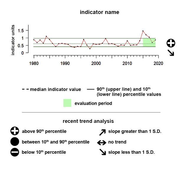
Resources
West Hawaii Integrated Ecosystem Assessment Ecosystem Status Report
The Ecosystem Status Report summarizes a suite of ecosystem indicators that track the status of the region’s marine ecosystem.

Papahānaumokuākea Marine National Monument 2020 Condition Report
This “condition report” provides a summary of resources in the Papahānaumokuākea Marine National Monument, which is co-managed by National Oceanic and Atmospheric Administration, the U.S. Fish and Wildlife Service and the State of Hawaii.

Fagatele Bay National Marine Sanctuary condition report
This report provides a summary of resources in the National Oceanic and Atmospheric Administration's Fagatele Bay National Marine Sanctuary, pressures on those resources, the current condition and trends, and management responses to the pressures that threaten the integrity of the marine environment.

NOAA Coral Reef Conservation Program
The National Oceanic and Atmospheric Administration (NOAA) Coral Reef Conservation Program is investing approximately $4.5 million of its annual operating budget to support a National Coral Reef Monitoring Plan (NCRMP) for biological, physical, and socioeconomic monitoring throughout the U.S. Pacific, Atlantic, and Caribbean coral reef areas.

Pacific Islands Ocean Observing System (PacIOOS)
The Pacific Islands Ocean Observing System (PacIOOS) aims to promote a safe, healthy and productive ocean and resilient coastal zone, PacIOOS collects real-time data on ocean conditions, forecasts future events, and develops user-friendly tools to access this information. In collaboration with a large network of partners, PacIOOS helps inform decision-making in Pacific communities on a daily basis.

NOAA Environmental Response Management Application (ERMA): Regional Portals
The Environmental Response Management Application is a web-based Geographic Information System (GIS) tool that assists emergency responders and environmental resource managers in dealing with incidents that may adversely impact the environment.
Hawaiian Islands Humpback Whale National Marine Sanctuary 2010 Condition Report
The Hawaiian Islands Humpback Whale National Marine Sanctuary (sanctuary) was designated to protect the humpback whale (Megaptera novaeangliae) and its habitat in Hawai'i. The sanctuary enables citizens and government to work collectively on safeguarding humpback whale breeding and calving range in waters around the main Hawaiian Islands.

Marine Biogeographic Assessment of the Main Hawaiian Islands
The state of Hawai'i is working to develop local renewable energy sources to reduce its dependence on fossil fuels. Most of the State's potential renewable energy resources (notably, wind) are located in federal waters from 3 to 200 nm offshore. The Bureau of Ocean Energy Management (BOEM) regulates the leasing, construction and operation of most renewable energy projects in federal waters, and is required to evaluate potential human, coastal and marine impacts from these projects. BOEM partnered with the National Oceanic and Atmospheric Administration's (NOAA) National Centers for Coastal Ocean Science (NCCOS) to gather biogeographic information in support of this evaluation around the Main Hawaiian Islands (MHI).