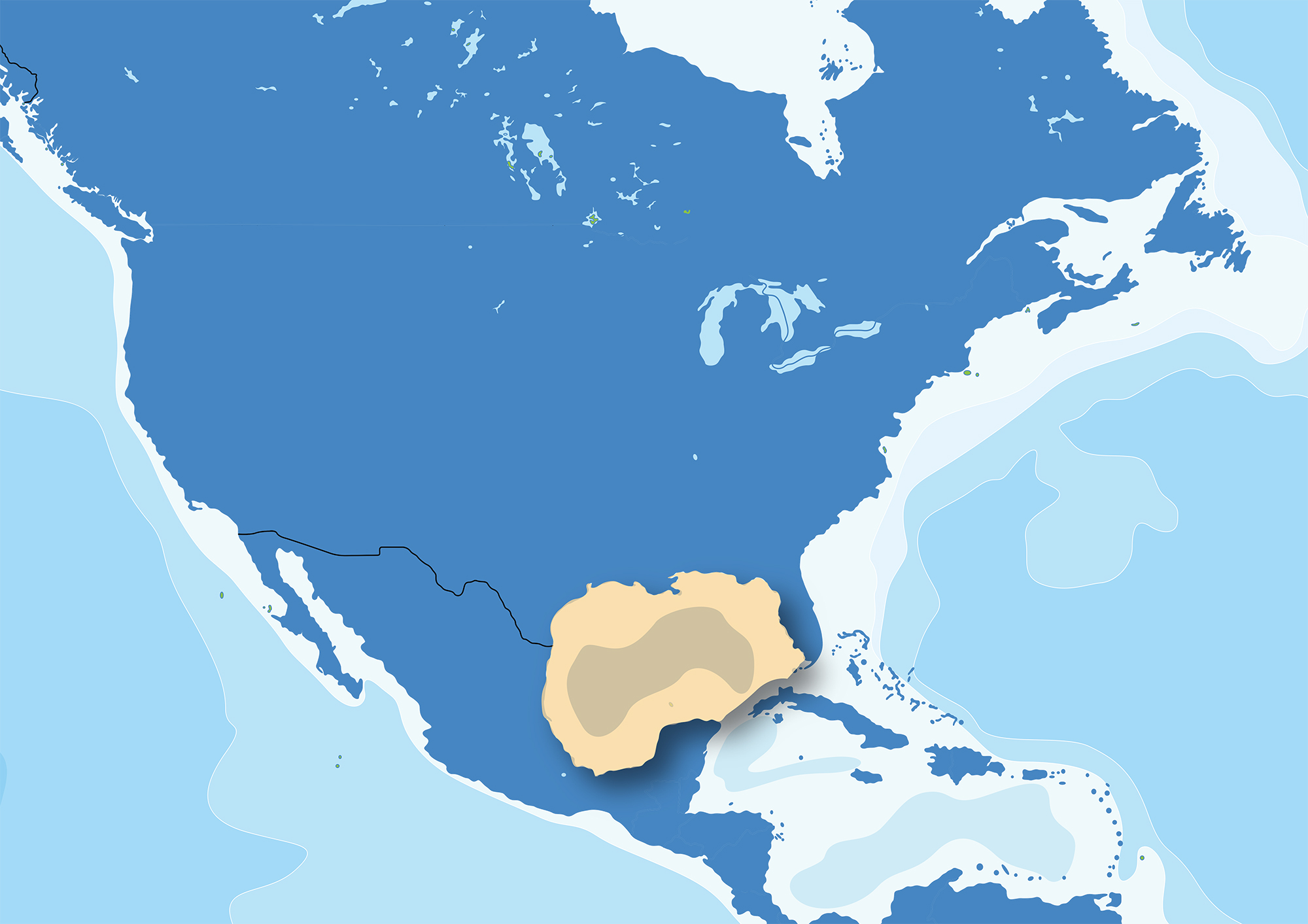
The Gulf of Mexico is a 218,000 square mile semi-enclosed, oceanic basin connected to the Atlantic Ocean by the Straits of Florida and to the Caribbean Sea by the Yucatan Channel. Many important watersheds, such as the Mississippi river, drain into the Gulf of Mexico. Many important species are found in the gulf such as red snappers, manatees, and
The region experiences some of the most severe weather in the world, including major hurricanes, tornadoes and thunderstorms. 17.2 million acres of marsh and nearly 30,000 miles of tidal shoreline draw millions of tourists to this area every year.
There are numerous threats to Gulf ecosystems, including one of the world’s largest areas of hypoxia, or “dead zone.” Each year, the dead zone sharply affects the region’s seafood production, illustrating the enormity and complexity of the threats facing the region’s ecosystem and, subsequently, the region’s economy.
Approximately half of total U.S. petroleum refining and natural gas processing capacity is located along the Gulf coast. This provides billions of dollars to the regional economy. Ship building and shipping are also multi-billion dollar industries, with two of the largest ports in the world, Houston and New Orleans, in the region.
Recreation, leisure, and tourism industries contribute significantly to the Gulf economy employing millions of people. The Gulf of Mexico supports some of the largest recreational and valuable commercial fisheries in the nation. These benefits bring a rising population, creating notable pressures on the very natural resources that provide the economic engine for the region.
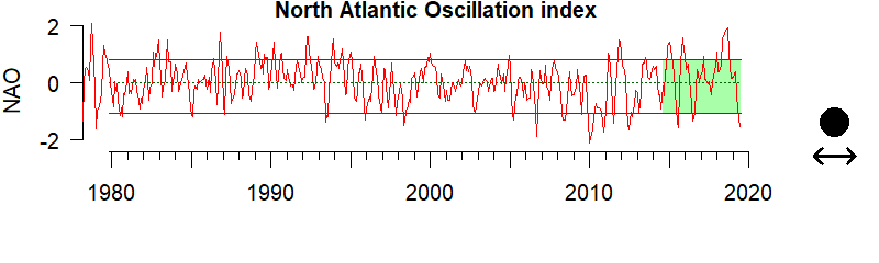
North Atlantic Oscillation (NAO)
.
Description of time series:
Positive NAO values mean significantly warmer winters over the upper Midwest and New England and negative NAO values can mean cold winter outbreaks and heavy snowstorms. During the last five years, the NAO indicator shows no significant trend.
Description of gauge:
The unitless two-way gauge depicts whether the average of the last 5 years of data for the climate indicator is above or below the median value of the entire time series. High values in either direction mean extreme variation from the median value of the entire time series.
Description of North Atlantic Oscillation (NAO):
The North Atlantic Oscillation (NAO) Index measures the relative strengths and positions of a permanent low-pressure system over Iceland (the Icelandic Low) and a permanent high-pressure system over the Azores (the Azores High). When the index is positive (NAO+) significantly warmer winters can occur over the upper Midwest and New England. On the East Coast of the United States a NAO+ can also cause increased rainfall, and thus warmer, less saline surface water. This prevents nutrient-rich upwelling, which reduces productivity. When the NAO index is negative, the upper central and northeastern portions of the United States can incur winter cold outbreaks and heavy snowstorms. We present data for the Northeast, Southeast, Gulf of Mexico, and Caribbean regions.
This climate condition impacts people and ecosystems across the globe and each of the indicators presented here. Interactions between the ocean and atmosphere alter weather around the world and can result in severe storms or mild weather, drought, or flooding. Beyond “just” influencing the weather and ocean conditions, these changes can produce secondary results that influence food supplies and prices, forest fires and flooding, and create additional economic and political consequences.
Data:
Climate indicator data was accessed from the NOAA Climate Prediction Center (https://www.cpc.ncep.noaa.gov/data/teledoc/nao.shtmlftp://ftp.cpc.ncep.noaa.gov/wd52dg/data/indices/nao_index.tim). The data plotted are unitless anomalies and averaged across a given region.
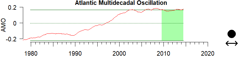
Atlantic Multidecadal Oscillation (AMO)
.
Description of time series:
Positive AMO values indicate the warm phase and negative AMO values indicate the cold phase. During the last five years, the AMO indicator shows no significant trend.
Description of gauge:
The unitless two-way gauge depicts whether the average of the last 5 years of data for the climate indicator is above or below the median value of the entire time series. High values in either direction mean extreme variation from the median value of the entire time series.
Description of Atlantic Multidecadal Oscillation (AMO):
The Atlantic Multidecadal Oscillation is a series of long-duration changes in the North Atlantic sea surface temperature, with cool and warm phases that may last for 20-40 years. Most of the Atlantic between the equator and Greenland changes in unison. Some areas of the North Pacific also seem to be affected.
This broadscale climate condition affects air temperatures and rainfall over much of the Northern Hemisphere. It is also related to major droughts in the Midwest and the Southwest of the U.S. In the warm phase, these droughts tend to be more frequent and/or severe. Vice-versa for the cold phase. During the warm phases the number of tropical storms that mature into severe hurricanes is much greater than during cool phases. We present data for the Northeast, Southeast, and Gulf of Mexico regions.
This climate condition impacts people and ecosystems across the globe and each of the indicators presented here. Interactions between the ocean and atmosphere alter weather around the world and can result in severe storms or mild weather, drought, or flooding. Beyond “just” influencing the weather and ocean conditions, these changes can produce secondary results that influence food supplies and prices, forest fires and flooding, and create additional economic and political consequences.
Data:
Climate indicator data was accessed from the NOAA Climate Prediction Center (https://www.cpc.ncep.noaa.gov/data/teledoc/nao.shtmlftp://ftp.cpc.ncep.noaa.gov/wd52dg/data/indices/nao_index.tim). The data plotted are unitless anomalies and averaged across a given region.
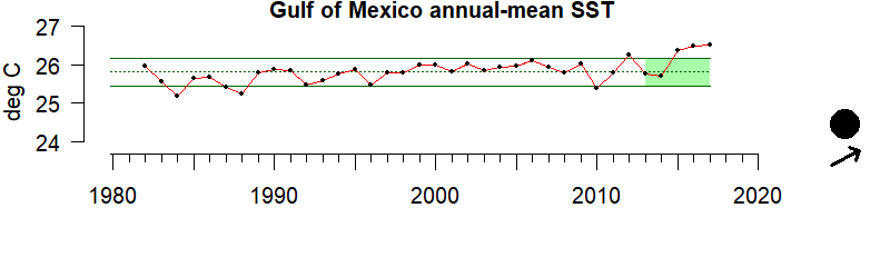
Sea Surface Temperature
.
Description of time series:
The time series shows the integrated sea surface temperature for this entire region. During the last five years there has been a positive trend and values have remained within the 10th and 90th percentiles.
Description of gauge:
This gauge does not show actual mean temperatures, but rather the gauge depicts the average of the last 5 years of data for Sea Surface Temperature relative to the median value of the entire time series. A gauge indicating 75 or greater indicates warmer than average temperatures over the past 5 years, whereas a gauge indicating 25 or less indicates cooler than average temperatures over the time period. The current value indicates that sea surface temperature is near the hotter end of what has been observed. Persistently warm conditions such as these can result in profound changes to the regional ecosystem.
Description of Sea Surface Temperature:
Sea Surface Temperature (SST) is defined as the average temperature of the top few millimeters of the ocean. This temperature impacts the rate of all physical, chemical, and most biological processes occurring in the ocean. Sea Surface Temperature is globally monitored by sensors on satellites, buoys, ships, ocean reference stations, AUVs and other technologies.
Sea Surface Temperature monitoring tells us how the ocean and atmosphere interact, as well as providing fundamental data on the global climate system. This information also aids us in weather prediction i.e. identifying the onset of El Niño and La Niña cycles - multiyear shifts in atmospheric pressure and wind speeds. These shifts affect ocean circulation, global weather patterns, and marine ecosystems. Sea Surface Temperature anomalies have been linked to shifting marine resources. With warming temperatures, we observe the poleward movements of fish and other species. Temperature extremes - both ocean heatwaves and cold spells, have been linked to coral bleaching as well as fishery and aquaculture mortality. We present annual average SST in all regions.
Data:
The sea surface temperature were accessed from (https://www.ncdc.noaa.gov/oisst). The data are plotted in degrees Celsius.
Sea level
Coastal sea level from tide gauges
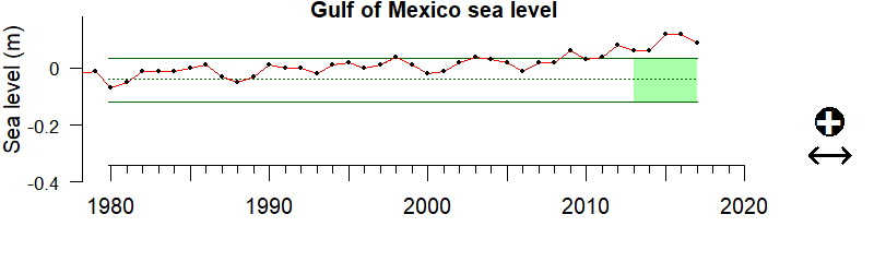
Sea level varies due to the force of gravity, the Earth’s rotation and irregular features on the ocean floor. Other forces affecting sea levels include temperature, wind, ocean currents, tides, etc. With 40 percent of Americans living in densely populated coastal areas, having a clear understanding of sea level trends is critical to societal and economic well being.
Measuring and predicting sea levels, tides and storm surge are important for determining coastal boundaries, ensuring safe shipping, and emergency preparedness, etc. NOAA monitors sea levels using tide stations and satellite laser altimeters. Tide stations around the globe tell us what is happening at local levels, while satellite measurements provide us with the average height of the entire ocean. Taken together, data from these sources are fed into models that tell us how our ocean sea levels are changing over time. For this site, data from tide stations around the US were combined to create regionally averaged records of sea-level change since 1980. We present data for all regions.
Chlorophyll-a
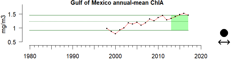
Description of time series:
During the last five years the chlorophyll a indicator shows no significant trend.
Description of gauge:
The gauge value of 80 indicates that over the last five years, average chlorophyll a has been much higher than the median value.
Description of Chlorophyll a:
At the base of most marine food webs are microscopic plants, called phytoplankton - which also produce nearly half of the Earth’s oxygen. One way we measure the amount of phytoplankton in the ocean is via a pigment that phytoplankton produce - chlorophyll a. Using ocean color sensors on satellites, we can measure the amount of chlorophyll a in surface waters. Environmental and oceanographic factors continuously influence the abundance, composition, spatial distribution, and productivity of phytoplankton. Tracking the amount of phytoplankton in the ocean gives us the status of the base of the food web, and how much food is available for other animals to grow. Changes in the amount of phytoplankton in the ocean are part of the natural seasonal cycle, but can also indicate an ecosystem’s response to a major external disturbance.
Overall Scores mean the following:
- 0 - 10: “significantly lower” the long term median state
- 10 - 25: “considerably lower” the long term median state
- 25 - 50: “slightly lower” the long term median state
- 50: the long term median state
- 50 - 75: “slightly above” the long term median state
- 75 - 90 “considerably above” the long term median state
- 90 - 100: “significantly higher” the long term median state
High values of Chlorophyll a can be good (lots of big nutrious diatoms) or bad (Harmful Algal Blooms), depending on the species present.
Data:
Chlorophyll a data were obtained from the NOAA Fisheries Coastal & Oceanic Plankton Ecology, Production, & Observations Database. Measurements of ocean chlorophyll concentration were combined from both the SeaWiFS and MODIS-Aqua "ocean color" datasets and binned at 0.5 x 0.5 degree latitude-longitude boxes, annual averages for each year calculated from the average of all monthly means in that year, and the annual mean was calculated as the average of all annual means. Source: https://www.st.nmfs.noaa.gov/copepod/about/about-copepod.html.
Zooplankton
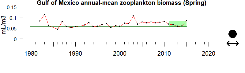
Description of time series:
During the last five years the zooplankton biomass indicator shows no significant trend.
Description of gauge:
The gauge value of 47 indicates that over the last five years, average zooplankton biomass has been close to the median value.
Description of Zooplankton:
Zooplankton are a diverse group of animals found in oceans, bays, and estuaries. By eating phytoplankton, and each other, zooplankton play a significant role in the transfer of materials and energy up the oceanic food web (e.g., fish, birds, marine mammals, humans.) Like phytoplankton, environmental and oceanographic factors continuously influence the abundance, composition and spatial distribution of zooplankton. These include the abundance and type of phytoplankton present in the water, as well as the water’s temperature, salinity, oxygen, and pH. Zooplankton can rapidly react to changes in their environment. For this reason monitoring the status of zooplankton is essential for detecting changes in, and evaluating the status of ocean ecosystems. We present the annual average total biovolume of zooplankton in the Alaska, California Current, Gulf of Mexico and Northeast regions.
Overall Scores mean the following:
High values of zooplankton can be good (lots of lipid rich colder water species) or bad (lots of lipid poor warmer water species), depending on the region.
- 0 - 10: The five-year zooplankton biomass average is very low compared to the median value.
- 10 - 25: The five-year zooplankton biomass average is much lower than the median value.
- 25 - 50: The five-year zooplankton biomass average is lower than the median value.
- 50: The five-year zooplankton biomass average equals the median value.
- 50 - 75: The five-year zooplankton biomass average is higher than the median value.
- 75 - 90: The five-year zooplankton biomass average is much higher than the median value.
- 90 - 100: The five-year zooplankton biomass average is very high compared to the median value.
Data:
Zooplankton data for each region were obtained from the NOAA Fisheries Coastal & Oceanic Plankton Ecology, Production, & Observations Database, an integrated data set of quality-controlled, globally distributed plankton biomass and abundance data with common biomass units and served in a common electronic format with supporting documentation and access software. Source: https://www.st.nmfs.noaa.gov/copepod/about/about-copepod.html
Coral reefs
Flower Garden Banks

Description of gauge:
The Flower Garden Banks score a 89, meaning they are ranked good with most indicators meeting reference values.
Description of Flower Garden Banks:
The East and West Flower Garden Banks are submerged topographic features off the shores of Texas and Louisiana in the Gulf of Mexico. Rising from over 150 m depth to 17 m below the sea surface, they harbor relatively deep coral reef ecosystems. They were first discovered in the early 1900s and designated as part of the Flower Garden Banks National Marine Sanctuary in 1992. Flower Garden Banks combines data collected from both East and West Flower Garden Banks into a single report. The total coral reef hardbottom habitat less than 30 meters in depth that was monitored for Flower Garden Banks is 0.898 square kilometers.
How Coral Reef indicator data are compiled and scored:
NOAA’s National Coral Reef Monitoring Program defines four main monitoring data themes in its monitoring plan (NOAA, 2014). The four monitoring themes are fish, coral and algae, climate, and human connections, and each has associated indicators. Available data were used by experts to score appropriate indicators for each theme. Scores are calculated on a 0-100% scale, with descriptive words and narrative text accompanying each score.
Overall scores mean the following:
90-100% Very good: All or almost all indicators meet reference values.
80-89% Good: Most indicators meet reference values.
70-79% Fair: Some indicators meet reference values.
60-69% Impaired: Few indicators meet reference values.
0-59% Critical: Very few or no indicators meet reference values.
Source: 2020 Status Report Scoring Methodology for Atlantic Jurisdictions
Coral reefs
Florida
Description of gauge:
The Florida coral reef score a 69, meaning they are ranked impaired with few indicators meeting reference values.
Description of Florida:
Florida’s coral reef extends from Martin County on the Atlantic Coast of Florida through the Keys to the Dry Tortugas in the Gulf of Mexico. Florida’s coral reef is the only coral reef found along the coast of the continental United States. It was divided into three sub-regions to evaluate condition. The three regions are Southeast Florida, Florida Keys, and Dry Tortugas.
How Coral Reef indicator data are compiled and scored:
The coral reef ecosystem scores shown here were analyzed using data from the National Coral Reef Monitoring Program (NCRMP). NCRMP collects data in all U.S. coral reef regions in four themes: benthic (corals and algae), reef fish, climate (ocean acidification and thermal stress), and human connections (socioeconomic surveys). The scores you see for each region are composite scores from all four themes assessed together and rolled into one overall score.
Overall scores mean the following:
90-100% Very good: All or almost all indicators meet reference values.
80-89% Good: Most indicators meet reference values.
70-79% Fair: Some indicators meet reference values.
60-69% Impaired: Few indicators meet reference values.
0-59% Critical: Very few or no indicators meet reference values.
Source: 2020 Status Report Scoring Methodology for Atlantic Jurisdictions
Forage fish
Menhaden biomass
Description of time series:
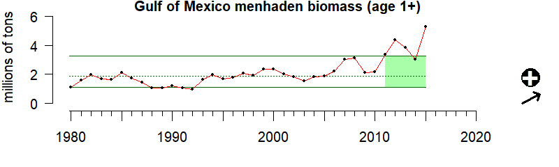
During the last five years the forage fish biomass shows a significant upward trend and is above the 90th percentile.
Description of gauge:
The Gauge value of 94 indicates that over the last five years, the forage fish biomass is very high compared to the median value.
Description of forage fish:
Forage fish or otherwise known as small pelagics are fish and invertebrates (like squids) that inhabit - the pelagic zone - the open ocean. The number and distribution of pelagic fish vary regionally, depending on multiple physical and ecological factors i.e. the availability of light, nutrients, dissolved oxygen, temperature, salinity, predation, abundance of phytoplankton and zooplankton, etc. Small pelagics are known to exhibit “boom and bust” cycles of abundance in response to these conditions. Examples include anchovies, sardines, shad, menhaden and the fish that feed on them
Small pelagic species are often important to fisheries and serve as forage for commercially and recreationally important fish, as well as other ecosystem species (e.g. seabirds and marine mammals). They are a critical part of marine food webs and important to monitor because so many other organisms depend on them. We present the annual total biomass of small pelagics/forage fish in the Alaska, California Current, and Northeast regions, as well as selected taxa in the Gulf of Mexico region.
Overall Scores means the following:
- 0 - 10: The five-year forage fish small pelagics average is very low compared to the median value.
- 10 - 25: The five-year forage fish small pelagics average is much lower than the median value.
- 25 - 50: The five-year forage fish small pelagics average is lower than the median value.
- 50: The five-year forage fish small pelagics average equals the median value.
- 50 - 75: The five-year forage fish small pelagics average is higher than the median value.
- 75 - 90: The five-year forage fish small pelagics average is much higher than the median value.
- 90 - 100: The five-year forage fish small pelagics average is very high compared to the median value.
Data:
Data for forage fish and small pelagics were obtained from regional NOAA Integrated Ecosystem Assessment Program teams that produce indicators and Ecosystem Status Report. For more information https://www.integratedecosystemassessment.noaa.gov/
Seabirds
Description of time series:
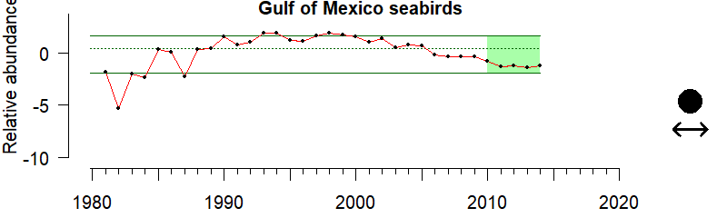
During the last five years the seabird relative abundance shows no significant trend.
Description of gauge:
The Gauge value of 26 indicates that over the last five years, the seabird relative abundance is much lower than the median value.
Description of Seabirds:
Seabirds are a vital part of marine ecosystems and valuable indicators of an ecosystem’s status. Seabirds are attracted to fishing vessels and frequently get hooked or entangled in fishing gear, especially longline fisheries. This is a common threat to seabirds. Depending on the geographic region, fishermen in the United States often interact with albatross, cormorants, gannet, loons, pelicans, puffins, gulls, storm-petrels, shearwaters, terns, and many other species. We track seabirds because of their importance to marine food webs, but also as an indication of efficient fishing practices. We present estimates of seabird abundance in the Alaska, California Current, Gulf of Mexico and Northeast regions.
Overall Scores means the following:
- 0 - 10: The five-year seabirds average is very low compared to the median value.
- 10 - 25: The five-year seabirds average is much lower than the median value.
- 25 - 50: The five-year seabirds average is lower than the median value.
- 50: The five-year seabirds average equals the median value.
- 50 - 75: The five-year seabirds average is higher than the median value.
- 75 - 90: The five-year seabirds average is much higher than the median value.
- 90 - 100: The five-year seabirds average is very high compared to the median value.
Data:
Data for Alaska, California Current, and the Gulf of Mexico were obtained from the regional NOAA Integrated Ecosystem Assessment Program teams that produce indicators and Ecosystem Status Report. For more information see https://www.integratedecosystemassessment.noaa.gov/. Seabird count and transect length data for the Northeast were extracted from the Atlantic Marine Assessment Program for Protected Species (AMAPPS) annual reports. Counts were summed and divided by the sum of the transect length in nautical miles. For more information see https://www.nefsc.noaa.gov/psb/AMAPPS/
Overfished stocks
.
Description of time series:
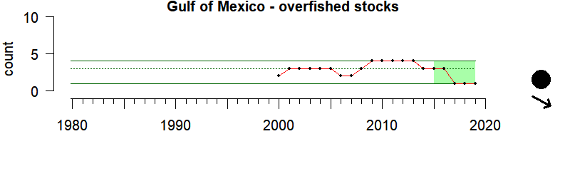
During the last five years the number of overfished stocks shows a significant downward trend.
Description of gauge:
The Gauge value of 15 indicates that over the last five years, the number of overfished stocks is much lower than the median value.
Description of Overfished stocks:
Fish play an important role in marine ecosystems, supporting the ecological structure of many marine food webs. Caught by recreational and commercial fisheries, fish support significant parts of coastal economies, and can play an important cultural role in many regions. To understand the health of fish populations - as well as their abundance and distribution, we regularly assess fish stocks - stock assessments. Assessments let us know if a stock is experiencing overfishing or if it is overfished i.e. how much catch is sustainable while maintaining a healthy stock. And, if a stock becomes depleted, stock assessments can help determine what steps may be taken to rebuild it to sustainable levels. Understanding stock assessments helps measure how well we’re managing and recovering fish stocks over time. We present the number of overfished stocks by year in all regions.
Overall Scores mean the following:
High values for overfished stocks are bad, low numbers are good.
- 0 - 10: The five-year overfished stock status average is very low compared to the median value.
- 10 - 25: The five-year overfished stock status average is much lower than the median value.
- 25 - 50: The five-year overfished stock status average is lower than the median value.
- 50: The five-year overfished stock status average equals the median value.
- 50 - 75: The five-year overfished stock status average is higher than the median value.
- 75 - 90: The five-year overfished stock status average is much higher than the median value.
- 90 - 100: The five-year overfished stock status average is very high compared to the median value.
Data:
Data were obtained (28 Aug 2019) from the NOAA Fisheries Fishery Stock Status website https://www.fisheries.noaa.gov/national/population-assessments/fishery-stock-status-updates. Stocks that met the criteria for overfished status were summed by year for each region.
Threatened/ endangered marine mammals
Endangered Species Act threatened/ endangered species
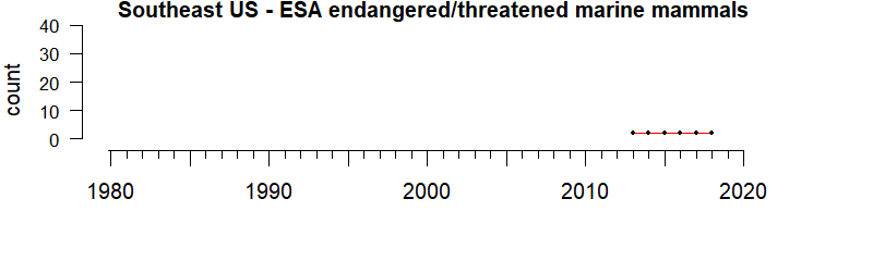
Description of time series:
Trend analysis was not appropriate for ESA data.
Description of gauge:
The Gauge value of 50 indicates that over the last five years, ESA threatened or endangered marine mammals average is the median value.
Description of Threatened and Endangered Marine mammals:
Some marine mammals face significant threats. The Endangered Species Act (ESA) aims to conserve endangered and threatened species and the ecosystems they depend on. Under the ESA, a species is considered endangered if it is in danger of extinction throughout all or a significant portion of its range, or threatened if it is likely to become endangered in the foreseeable future. We present the annual number of threatened and endangered marine mammals in all regions except the Caribbean. Data for the Southeast and Gulf of Mexico regions are combined.
Overall Scores mean the following:
High values of ESA threatened and endangered species are bad, low numbers are good.
- 0 - 10: The five-year ESA threatened or endangered marine mammals average is very low compared to the median value.
- 10 - 25: The five-year ESA threatened or endangered marine mammals is much lower than the median value.
- 25 - 50: The five-year ESA threatened or endangered marine mammals average is lower than the median value.
- 50: The five-year ESA threatened or endangered marine mammals average equals the median value.
- 50 - 75: The five-year ESA threatened or endangered marine mammals average is higher than the median value.
- 75 - 90: The five-year ESA threatened or endangered marine mammals average is much higher than the median value.
- 90 - 100: The five-year ESA threatened or endangered marine mammals average is very high compared to the median value.
Data:
Summary data tables from the NOAA Fisheries Protected Resources Species Information System were obtained from the database manager 3 April 2020. The number of ESA threatened and endangered species were summed for each region by year.
Strategic/ depleted marine mammal stocks
Marine Mammal Protection Act strategic/ depleted stocks
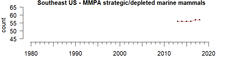
Description of time series:
Trend analysis was not appropriate for MMPA data.
Description of gauge:
The Gauge value of 50 indicates that over the last five years, MMPA strategic and depleted marine mammals average is the median value.
Description of marine mammals depleted stocks (MMPA):
A strategic stock is defined by the Marine Mammal Protection Act as a marine mammal stock—For which the level of direct human-caused mortality exceeds the potential biological removal level; Which, based on the best available scientific information, is declining and is likely to be listed as a threatened species under the Endangered Species Act within the foreseeable future; or Which is listed as a threatened or endangered species under the ESA, or is designated as depleted under the MMPA.
A depleted stock is defined by the MMPA as any case in which—The Secretary of Commerce, after consultation with the Marine Mammal Commission and the Committee of Scientific Advisors on Marine Mammals established under MMPA title II, determines that a species or population stock is below its optimum sustainable population; a State, to which authority for the conservation and management of a species or population stock is transferred under section 109, determines that such species or stock is below its optimum sustainable population; or A species or population stock is listed as an endangered species or a threatened species under the ESA. We present the annual number of strategic and depleted marine mammals in all regions except the Caribbean. Data for the Southeast and Gulf of Mexico regions are combined.
Overall Scores mean the following:
- 0 - 10: The five-year MMPA strategic and depleted marine mammals average is very low compared to the median value.
- 10 - 25: The five-year MMPA strategic and depleted marine mammals average is much lower than the median value.
- 25 - 50: The five-year MMPA strategic and depleted marine mammals average is lower than the median value.
- 50: The five-year MMPA strategic and depleted marine mammals average equals the median value.
- 50 - 75: The five-year MMPA strategic and depleted marine mammals average is higher than the median value.
- 75 - 90: The five-year MMPA strategic and depleted marine mammals average is much higher than the median value.
- 90 - 100: The five-year MMPA strategic and depleted marine mammals average is very high compared to the median value.
Data:
Data methods Summary data tables from the NOAA Fisheries Protected Resources Species Information System were obtained from the database manager 3 April 2020. The number of MMPA strategic and depleted stock species were summed for each region by year.
Unusual Mortality Events
significant die-offs in a marine mammal population
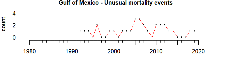
Description of time series:
Trend analysis was not appropriate for UME data.
Description of gauge:
The gauge value of 27 indicates that over the last five years, average marine mammal unusual mortality events have been lower than average.
Description of Unusual Mortality events:
Marine mammals are important parts of marine ecosystems. Sometimes we observe significant die-offs in a marine mammal population - also called unusual mortality events (UMEs). A UME is defined as "a stranding that is unexpected; involves a significant die-off of any marine mammal population; and demands immediate response." UMEs are often caused by ecological factors (e.g. changes in ocean conditions or food sources), biotoxins, infectious disease, and human interactions, but in some cases the cause cannot be determined. Some unusual mortality events occur over a period of months and others last for years. Understanding and investigating marine mammal UMEs is crucial because they can be indicators of ocean health, giving insight into larger environmental issues, which may also have implications for human health. We present the number of unusual marine mammal mortality events in a given year in all the Alaska, Pacific Islands, California Current, Gulf of Mexico, Southeast, and Northeast regions.
Overall Scores mean the following:
High values for UME are bad, low values are good.
- 0 - 10: The five-year UME average is very low compared to the median value.
- 10 - 25: The five-year UME average is much lower than the median value.
- 25 - 50: The five-year UME average is lower than the median value.
- 50: The five-year UME average equals the median value.
- 50 - 75: The five-year UME average is higher than the median value.
- 75 - 90: The five-year UME average is much higher than the median value.
- 90 - 100: The five-year UME average is very high compared to the median value.
Data:
Unusual mortality event (UME) data for marine mammals were accessed from the NOAA Fisheries Active and Closed Unusual Mortality Events website (https://www.fisheries.noaa.gov/national/marine-life-distress/active-and-closed-unusual-mortality-events). A value of 1 was assigned for each UME (open and closed) reported as occurring for any portion of a given year and the values were summed by year for each region. For UMEs where the date range was not indicated, a value of 1 was applied only for the year the UME was declared.
Coastal population
.
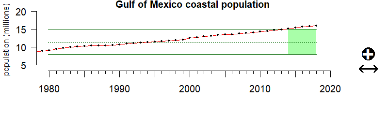
Description of time series:
The 2014 – 2018 average coastal population along the Gulf of Mexico was substantially above historic levels, although the recent trend is not different from historical trends.
Description of gauge:
The 2014 – 2018 average coastal population along the Gulf of Mexico was greater than 94% of all population levels between 1970 to 2018, again highlighting the substantial growth in the coastal population of this region.
Description of Coastal Population:
While marine ecosystems are important for people all across the country, they are essential for people living in coastal communities. The population density of coastal counties is over six times greater than inland counties. In the U.S. coastal counties make up less than 10 percent of the total land area (not including Alaska), but account for 39 percent of the total population. From 1970 to 2010, the population of these counties increased by almost 40% and are projected to increase by over 10 million people or 8+% into the 2020s.
The population density of an area is an important factor for economic planning, emergency preparedness, understanding environmental impacts, resource demand, and many other reasons. Thus, this indicator is important to track. We present the number of residents within all regions.
Extreme Gauge values:
A value of zero on the gauge means that the average coastal population over the last 5 years of data was below any annual population level up until that point, while a value of 100 would indicate the average over that same period was above any annual population level up until that point.
Data:
Coastal population data was retrieved from the Census Bureau’s county population totals, filtered to present coastal counties using the Census Bureau’s list of coastal counties within each state. Coastal county populations were then summed within each region for reporting purposes.
Coastal tourism
.
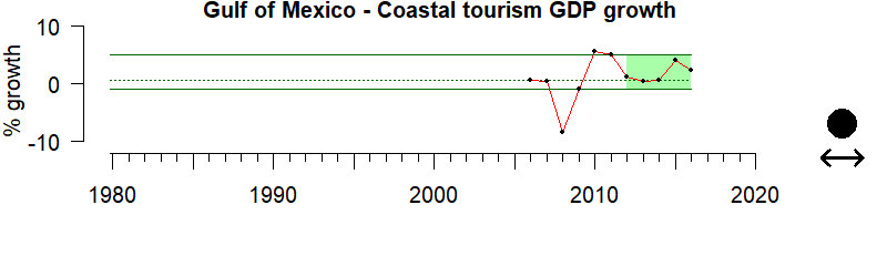
Description of time series:
The growth in the value of coastal tourism along the Gulf of Mexico varies considerably across time, with an upward trend although the last 5 years of growth shows no difference from historical patterns.
Description of gauge:
The value of coastal tourism along the Gulf of Mexico grew at a rate of 2.2% between 2015-2016, faster than the rest of the regional economy, which grew 0.2%, and other ocean sectors, which decreased 13.5% over that same time period.
Description of Coastal Tourism:
Coastal tourism Gross Domestic Product is the total measure (in billions of dollars) of goods and services provided from tourism along the coast. U.S. coasts are host to a multitude of travel, tourism, and recreation activities. These provide social and economic benefits as well as impact the environment. As more and more communities turn to tourism for economic development, it becomes crucial to develop a sustainable tourism industry that is good for communities, the environment, and society more broadly. To accomplish this, we need data on the social and economic impacts of recreation and tourism, and its impacts on natural resources. We present the annual total change (in billions of dollars) of goods and services provided from tourism in the Gulf of Mexico, Mid-Atlantic, Northeast, Pacific Islands, Southeast, and California Current regions.
Extreme Gauge values:
A value of zero on the gauge means that the average coastal tourism over the last 5 years of data was below any annual coastal tourism level up until that point, while a value of 100 would indicate the average over that same period was above any annual coastal tourism level up until that point.
Data:
Coastal Tourism GDP data was taken from NOAA’s Office of Coastal Management Economics National Ocean Watch custom report building tool, with contextual data taken from the 2019 NOAA Report on the U.S. Ocean and Great Lakes Economy: Regional and State Profiles. Growth was estimated by subtracting the previous year’s Coastal Tourism GDP from the current year’s Coastal Tourism GDP, then dividing by the previous year’s Coastal Tourism GDP to present a percentage. All data was deflated to 2012 constant dollars using the Bureau of Economic Analysis’ chained dollar methodology.
Coastal employment
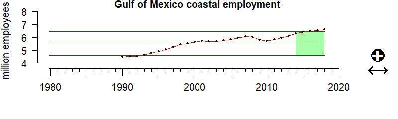
Description of time series:
Average coastal employment along the Gulf of Mexico between 2014 and 2018 was substantially above historical levels, although no trend is apparent over that same period.
Description of gauge:
The 2014 – 2018 average annual employment level along the Gulf of Mexico is greater than 90% of all employment levels between 1990 and 2018, indicating that employment levels over that period were high compared to historical levels.
Description of Coastal Employment:
Coastal employment numbers were downloaded from the U.S. Bureau of Labor Statistics’ quarterly census of employment and wages, filtered to present only coastal county values using the Census Bureau’s list of coastal counties within each state. Of note is that these data fail to include self-employed individuals. Coastal county employment numbers were then summed within each region for reporting purposes.
Extreme Gauge values:
A value of zero on the gauge means that the average coastal employment level over the last 5 years of data was below any annual employment level up until that point, while a value of 100 would indicate the average over that same period was above any annual employment level up until that point.
Data:
Coastal employment numbers were downloaded from the U.S. Bureau of Labor Statistics’ quarterly census of employment and wages, filtered to present only coastal county values using the Census Bureau’s list of coastal counties within each state. Of note is that these data fail to include self-employed individuals. Coastal county employment numbers were then summed within each region for reporting purposes.
Commercial fishery landings
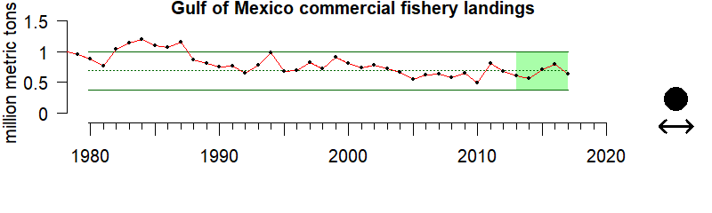
Description of time series:
Between 2013 and 2017, commercial landings from the Gulf of Mexico were similar to historic levels, and there is no recent trend apparent.
Description of gauge:
Between 2013 and 2017, average commercial landings from the Gulf of Mexico were greater than 40% of all annual landings from 1950 to 2017.
Description of Commercial Fishing (Landings and Revenue):
Commercial landings are the weight of, or revenue from, fish that are caught, brought to shore, processed, and sold for profit. It does not include sport or subsistence (to feed themselves) fishermen or for-hire sector, which earns its revenue from selling recreational fishing trips to saltwater anglers.
Commercial landings make up a major part of coastal economies. U.S. commercial fisheries are among the world’s largest and most sustainable; producing seafood, fish meal, vitamin supplements, and a host of other products for both domestic and international consumers.
The weight (tonnage), and revenue from the sale of commercial landings provides data on the ability of marine ecosystems to continue to supply these important products.
Extreme Gauge values:
A value of zero on the gauge means that the average revenue or landings over the last 5 years of data was below any annual value up until that point, while a value of 100 would indicate the average value over that same period was above any annual value up until that point.
Data:
Commercial landings and gross revenue were downloaded from the National Marine Fisheries Service’s annual commercial fisheries landings query tool which can be found at https://foss.nmfs.noaa.gov/apexfoss/f?p=215:200::::::. State pounds landed and revenue generated were aggregated to the appropriate region, and all revenue data was deflated to 2017 constant dollars using the Bureau of Labor Statistic’s Consumer Price Index (series CUUR0000SA0).
Commercial fishing revenue
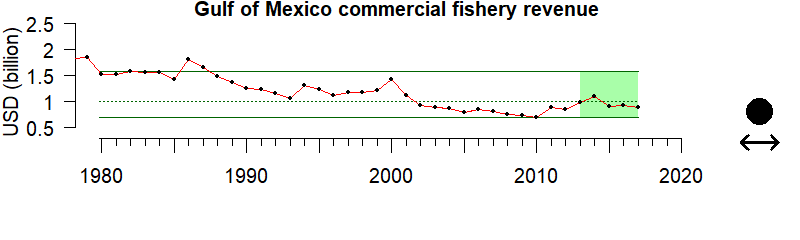
Description of time series:
Between 2013 and 2017, average annual commercial revenue from the Gulf of Mexico was not different than historical patterns, and there is no trend in values.
Description of gauge:
Between 2013 and 2017, average annual commercial revenue from the Gulf of Mexico was greater than 46% of all annual revenue from 1950 to 2017.
Description of Commercial Fishing (Landings and Revenue):
Commercial landings are the weight of, or revenue from, fish that are caught, brought to shore, processed, and sold for profit. It does not include sport or subsistence (to feed themselves) fishermen or for-hire sector, which earns its revenue from selling recreational fishing trips to saltwater anglers.
Commercial landings make up a major part of coastal economies. U.S. commercial fisheries are among the world’s largest and most sustainable; producing seafood, fish meal, vitamin supplements, and a host of other products for both domestic and international consumers.
The weight (tonnage), and revenue from the sale of commercial landings provides data on the ability of marine ecosystems to continue to supply these important products.
Extreme Gauge values:
A value of zero on the gauge means that the average revenue or landings over the last 5 years of data was below any annual value up until that point, while a value of 100 would indicate the average value over that same period was above any annual value up until that point.
Data:
Commercial landings and gross revenue were downloaded from the National Marine Fisheries Service’s annual commercial fisheries landings query tool which can be found at https://foss.nmfs.noaa.gov/apexfoss/f?p=215:200::::::. State pounds landed and revenue generated were aggregated to the appropriate region, and all revenue data was deflated to 2017 constant dollars using the Bureau of Labor Statistic’s Consumer Price Index (series CUUR0000SA0).
Recreational fishing effort
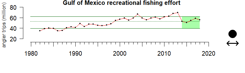
Description of time series:
Between 2013 and 2018, recreational fishing effort in the Gulf of Mexico is around historic levels. There is no trend apparent.
Description of gauge:
Between 2013 and 2018, the Gulf of Mexico’s average recreational fishing effort was greater than 57% of all recreational fishing effort from 1982 to 2018.
Description of Recreational Fishing (Effort and Harvest):
U.S. saltwater recreational fishing is an important source of seafood, jobs, and recreation for millions of anglers and for-hire recreational businesses. Recreational fishing effort is measured as “Angler Trips”, which is the number of recreational fishing trips people go on. Recreational fishing harvest is the number of fish caught and brought to shore on recreational fishing trips.
Recreational effort and harvest help us understand how recreational opportunities and seafood derived from our marine environment is changing over time. Fisheries managers use this data to set annual catch limits and fishing regulations, including season lengths, size, and daily catch limits. We present the total number of fish caught and angler trips annually for all marine fish in all regions.
Extreme Gauge values:
A value of zero on the gauge means that the average effort or harvest over the last 5 years of data was below any annual value up until that point, while a value of 100 would indicate the average value over that same period was above any annual value up until that point.
Data:
Recreational harvest and effort data pulled from National Summary Query at https://www.st.nmfs.noaa.gov/recreational-fisheries/data-and-documentation/queries/index Units of data are in Effort in Angler Days and Harvest in numbers of fish.
Recreational fishing harvest
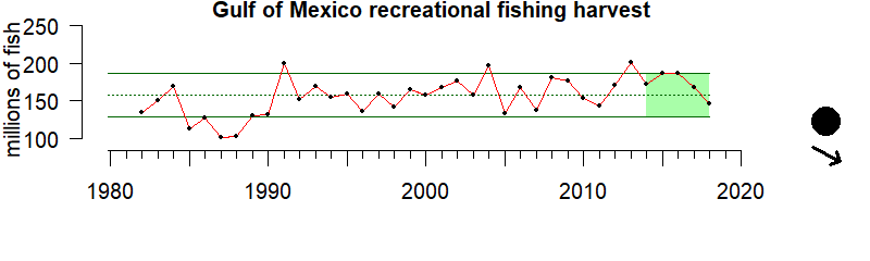
Description of time series:
Between 2013 and 2018, recreational harvest from Gulf of Mexico are around historic levels. There is a significant upward trend apparent.
Description of gauge:
Between 2013 and 2018, Gulf of Mexico’s average recreational landings were greater than 76% of all landings from 1982 to 2018.
Description of Recreational Fishing (Effort and Harvest):
U.S. saltwater recreational fishing is an important source of seafood, jobs, and recreation for millions of anglers and for-hire recreational businesses. Recreational fishing effort is measured as “Angler Trips”, which is the number of recreational fishing trips people go on. Recreational fishing harvest is the number of fish caught and brought to shore on recreational fishing trips.
Recreational effort and harvest help us understand how recreational opportunities and seafood derived from our marine environment is changing over time. Fisheries managers use this data to set annual catch limits and fishing regulations, including season lengths, size, and daily catch limits. We present the total number of fish caught and angler trips annually for all marine fish in all regions.
Extreme Gauge values:
A value of zero on the gauge means that the average effort or harvest over the last 5 years of data was below any annual value up until that point, while a value of 100 would indicate the average value over that same period was above any annual value up until that point.
Data:
Recreational harvest and effort data pulled from National Summary Query at https://www.st.nmfs.noaa.gov/recreational-fisheries/data-and-documentation/queries/index Units of data are in Effort in Angler Days and Harvest in numbers of fish.
Commercial fishing engagement
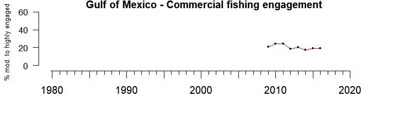
Description of time series:
There is not enough data to do trend analysis.
Description of gauge:
The 2012 – 2016 average percentage of commercially engaged communities along the Gulf of Mexico is greater than 25% of all engagement levels between 2009 and 2016 in that region, indicating that recent engagement levels are somewhat lower than historical levels.
Description of Fishing Engagement:
Recreational and commercial fishing engagement is measured by the presence of fishing activity in coastal communities. The commercial engagement index is measured through permits, fish dealers, and vessel landings. The data for recreational engagement indicators varies by state. A high rank within these indicates more engagement in fisheries. For details on both data sources and indicator development, please see https://www.fisheries.noaa.gov/national/socioeconomics/social-indicators-fishing-communities-0.
NOAA Monitors recreational and commercial fishing engagement to better understand the social and economic impacts of fishing policies and regulations on our nation’s vital fishing communities. This and other social indicators help assess a coastal community’s resilience. NOAA works with state and local partners to monitor these indicators. We present data from the Northeast, Southeast, Gulf of Mexico, California Current, Alaska, and Pacific Island regions.
Extreme Gauge values:
A value of zero on the gauge means that the average percentage of communities engaged in commercial or recreational fishing over the last 5 years of data was below any annual engagement level up until that point, while a value of 100 would indicate the average over that same period was above any engagement level up until that point.
Data:
Recreational and Commercial fishing engagement data is from the National Marine Fisheries Service’s social indicator data portal:https://www.st.nmfs.noaa.gov/data-and-tools/social-indicators/ The percentage of all communities in each region classified as medium, medium high, or highly engaged is presented for both recreational and commercial fishing.
Recreational fishing engagement
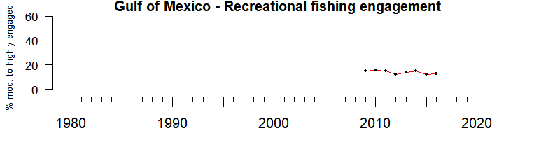
Description of time series:
There isn't enough data to do trend analysis. The Gulf of Mexico recreational engagement index is measured using shore, private vessel and for-hire vessel fishing activity estimates for western Florida to Mississippi. The index for Louisiana and Texas is measured using estimates for boat ramps, fishing piers, recreational vessels by homeport and recreational vessels by owner address.
Description of gauge:
The 2012 – 2016 average percentage of recreationally engaged communities along the Gulf of Mexico is greater than 38% of engagement levels between 2009 and 2016 in that region, indicating that recent engagement levels are similar to median historical levels.
Description of Fishing Engagement:
Recreational and commercial fishing engagement is measured by the presence of fishing activity in coastal communities. The commercial engagement index is measured through permits, fish dealers, and vessel landings. The data for recreational engagement indicators varies by state. A high rank within these indicates more engagement in fisheries. For details on both data sources and indicator development, please see https://www.fisheries.noaa.gov/national/socioeconomics/social-indicators-fishing-communities-0.
NOAA Monitors recreational and commercial fishing engagement to better understand the social and economic impacts of fishing policies and regulations on our nation’s vital fishing communities. This and other social indicators help assess a coastal community’s resilience. NOAA works with state and local partners to monitor these indicators. We present data from the Northeast, Southeast, Gulf of Mexico, California Current, Alaska, and Pacific Island regions.
Extreme Gauge values:
A value of zero on the gauge means that the average percentage of communities engaged in commercial or recreational fishing over the last 5 years of data was below any annual engagement level up until that point, while a value of 100 would indicate the average over that same period was above any engagement level up until that point.
Data:
Recreational and Commercial fishing engagement data is from the National Marine Fisheries Service’s social indicator data portal:https://www.st.nmfs.noaa.gov/data-and-tools/social-indicators/ The percentage of all communities in each region classified as medium, medium high, or highly engaged is presented for both recreational and commercial fishing.
Beach closures
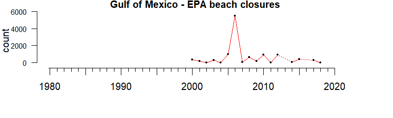
Interpretation of time series:
Trend analysis was not appropriate for BEACH Act data.
Interpretation of gauge:
A gauge was not appropriate for this data.
Description of beach closure:
Beach closures are the number of days when beach water and/or air quality is determined to be unsafe. Unsafe water and air quality may have significant impacts on human health, local economies, and the ecosystem. The Environmental Protection Agency (EPA) supports coastal states, counties and and tribes in monitoring beach water quality, and notifying the public when beaches must be closed. Beach water quality is determined by the concentration of bacteria in the water (either Enterococcus sp.or Escherichia coli).
The information presented is from states, counties, and tribes that submit data to the EPA Beach Program reporting database. Not all US beach closures are captured in this database. We present a summary of known EPA Beach Program closure days by year for Alaska, California Current, Gulf of Mexico, Northeast, Hawai’ian Islands, and the Southeast regions..
Gauge values
- 0 - 10: The five-year beach closure days average is very low compared to the median value.
- 10 - 25: The five-year beach closure days average is much lower than the median value.
- 25 - 50: The five-year beach closure days average is lower than the median value.
- 50: The five-year beach closure days average equals the median value.
- 50 - 75: The five-year beach closure days average is higher than the median value.
- 75 - 90: The five-year beach closure days average is much higher than the median value.
- 90 - 100: The five-year beach closure days average is very high compared to the median
Source and analysis of data:
Data obtained from the EPA BEACON website have been provided to EPA by the coastal and Great Lakes states, tribes and territories that receive grants under the BEACH Act. Data was refined to closure, by state or territory, by year. Data that were not identified to a water body or identified as inland water were not included. Data compiled by states or territory and combined in regions defined as IEA regions except PI includes Guam and Marianas. Caribbean and South Atlantic data stand alone. Not all beaches in a state or territory are monitored through the EPA BEACH Act. Data for beaches monitored by state and local municipalities is not included. Changes in the number of beach closure days may be driven by changes in the number of beaches monitored under the BEACH Act versus by state and local municipalities.
Billion-dollar disasters
Interpretation of time series:
The number of billion dollar disasters along the Gulf of Mexico is extremely variable over time, fluctuating between zero and thirteen disasters a year. The number of disasters over the past 5 years is substantially higher than historical levels of events, although the recent trend is not different from historical trends in the number of events.
Interpretation of gauge:
The average number of billion dollar disasters along the Gulf of Mexico over the last 5 years is higher than 93 percent of all annual disaster frequencies in that region.
Description of billion dollar disasters:
In the United States the number of weather and climate-related disasters exceeding 1 billion dollars has been increasing since 1980. These events have significant impacts to coastal economies and communities. The Billion Dollar Disaster indicator provides information on the frequency and the total estimated costs of major weather and climate events that occur in the United States. This indicator compiles the annual number of weather and climate-related disasters across seven event types. Events are included if they are estimated to cause more than one billion U.S. dollars in direct losses. The cost estimates of these events are adjusted for inflation using the Consumer Price Index (CPI) and are based on costs documented in several Federal and private-sector databases. We Present the total annual number of disaster events for all regions.
Extreme Gauge values
A value of zero on the gauge means that the average number of disasters over the last 5 years of data was below any annual level up until that point, while a value of 100 would indicate the average over that same period was above any annual number of disasters up until that point.
Source and analysis of data:
Billion dollar disaster event frequency data are taken from NOAA’s National Centers for Environmental Information. The number of disasters within each region were summed for every year of available data. Although the number is the count of unique disaster events within a region, the same disaster can impact multiple regions, meaning a sum across regions will overestimate the unique number of disasters.
Resources
Gulf of Mexico Ecosystem Status report
With the aim of supporting Ecosystem-Based Management, the Gulf of Mexico NOAA Integrated Ecosystem Assessment Program seeks to provide scientific knowledge of the Gulf of Mexico integrated ecosystem, and transfer that knowledge to scientists and managers. A suite of indicators was developed to represent key components of the GoM, and are presented in this website and report.
Gulf of Mexico Data Atlas
Launched in 2011, the Gulf of Mexico Data Atlas provides more than just maps. Links to data download sites provide easy access to each map's source data. Descriptions of the datasets accompany the maps and explains why the data are important to Gulf of Mexico coastal and marine ecosystems. Metadata records provide the complete details about how the data were collected. WMS and REST services allow for easy import of the map layers into desktop and web-based clients.
Flower Gardens Banks National Marine Sanctuary Condition Report
This "condition report" provides a summary of marine resources in the National Oceanic and Atmospheric Administration's Flower Garden Banks National Marine Sanctuary, pressures on those resources, current condition and trends, and management responses to the pressures that threaten the integrity of the marine environment.
NOAA Coral Reef Conservation Program
The National Oceanic and Atmospheric Administration (NOAA) Coral Reef Conservation
Program is investing approximately $4.5 million of its annual operating budget to support a
National Coral Reef Monitoring Plan (NCRMP) for biological, physical, and socioeconomic
monitoring throughout the U.S. Pacific, Atlantic, and Caribbean coral reef areas.
Gulf of Mexico Coastal Ocean Observing System (GCOOS)
The Gulf of Mexico Coastal Ocean Observing System Regional Association (GCOOS-RA) is a 501(c)3 organization responsible for developing a network of business leaders, marine scientists, resource managers, governmental and non-governmental organizations and other stakeholder groups that combine their data to provide timely information about our oceans — similar to the information gathered by the National Weather Service to develop weather forecasts.
Florida Keys National Marine Sanctuary Condition Report
This "condition report" provides a summary of resources in the National Oceanic and Atmospheric Administration's Florida Keys National Marine Sanctuary (sanctuary), pressures on those resources, current conditions and trends, and management responses to the pressures that threaten the integrity of the marine environment.
Florida Keys National Marine Sanctuary Ecosystem Status Report
This Ecosystem Status Report is compiled by NOAA’s Florida Keys Integrated Ecosystem Assessment Program (IEA) team, in collaboration with academic partners, Sanctuary resource managers and scientists, non governmental organizations, and other government and state agencies.
South Florida Ecosystem Restoration Indicators
This report is a digest of scientific findings about eleven system-wide ecological indicators in the South Florida Ecosystem.
MBON and the Sanctuaries MBON project
The Marine Biodiversity Observation Network (MBON) is a growing global initiative composed of regional networks of scientists, resource managers, and end-users working to integrate data from existing long-term programs to improve our understanding of changes and connections between marine biodiversity and ecosystem functions.
Gulf of Mexico Harmful Algal Bloom Forecast
In the Gulf of Mexico, some harmful algal blooms are caused by the rapid growth of the microscopic algae species Karenia brevis (commonly called red tide). Red tide can cause respiratory illness and eye irritation in humans. It can also kill marine life. Blooms are often patchy, so impacts vary by beach and throughout the day.
NOAA monitors conditions daily and issues twice-weekly forecasts for red tide blooms in the Gulf of Mexico and East Coast of Florida. You can find up-to-date information on where a bloom is located and a 3–4 day forecast for potential respiratory irritation by selecting a region below. This information may help you find an unaffected beach if you are visiting the coast.